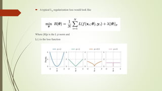
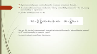
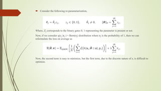
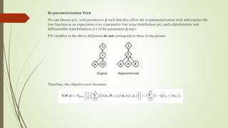
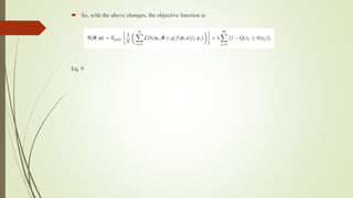
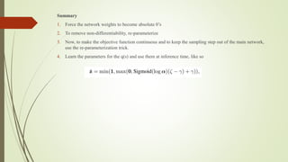
The document discusses the learning of sparse neural networks using l0 regularization, emphasizing its advantages in model compression and sparsification to combat overfitting. It describes the computational challenges posed by the non-differentiability of the l0 norm and introduces a re-parameterization approach that employs a continuous random variable to reformulate the loss function. The findings highlight the importance of optimizing network weights to achieve sparsity while maintaining differentiability through the re-parameterization trick.

1. Learning Sparse Neural Networks using
L0 Regularization
- Varun Reddy G

2. Neural Networks
 Very good function approximators and flexible
 Scales well
Some problems
1. Highly overparameterized
2. Can easily overfit.
One of the Solutions:
Model Compression and Sparsification

3.  A typical Lp regularization loss would look like
Where ||θ||p is the L p norm and
L(.) is the loss function

4.  L0 norm essentially means counting the number of non-zero parameters in the model.
 It penalizes all non-zero values equally, unlike other Lp norms which penalize on the value of θj causing
more shrinkage on higher values
So, now the error function looks like this
But, now this function is computationally intractable given non-differentiability and combinatorial nature of
the 2 |θ| possible states for the parameter vector θ
So, we reformulate to try and make it continuous.

5.  Consider the following re-parametarization,
Where, Zj corresponds to the binary gates 0, 1 representing the parameter is present or not.
Now, if we consider q(zj |πj ) = Bern(πj) distribution where πj is the probability of 1, then we can
reformulate the loss on average as
Now, the second term is easy to minimize, but the first term, due to the discrete nature of z, is difficult to
optimize.

6. Let s be a continuous random variable with a distribution q(s) and let the z’s be given by a hard-sigmoid
rectification of s
Hard-sigmoid
f(.) = min(1, max(0, .))
So, now z is given by
z = min(1, max(0, s))
This is equivalent to
z =
0 𝑖𝑓 𝑠 ≤ 0
1 𝑖𝑓 𝑠 ≥ 1
𝑠 𝑖𝑓 0 < 𝑠 < 1
So, if we look at the loss function, we have to penalize all the non-zero θ, so, the second term is
essentially the probability of s < 0, which is given out by the CDF Q(s)
Substituting these

7.  Our loss function becomes
where g(s) is our hard-sigmoid function.

8. Re-parameterization Trick
We can choose q(s), with parameters ɸ such that they allow the re-parameterization trick and express the
loss function as an expectation over a parameter free noise distribution p(ϵ) and a deterministic and
differentiable transformation f(.) of the parameters ɸ and ϵ
P.S variables in the above definition do not correspond to those in the picture
Therefore, the objective now becomes,

9. Choosing the q(s)
We are free to choose the q(s) and something that worked well in practice is a binary concrete random
variable distributed in (0, 1) with probability density qs (s| ɸ) and cumulative density Qs (s | ɸ).
The parameters of this distribution are ɸ = (log ⍺, β) where, log ⍺ is location and β is temperature.
We stretch this distribution to an interval (ɣ, 𝛿) such that ɣ < 0 and 𝛿 > 0 and apply hard-sigmoid on its
random samples

10.  So, with the above changes, the objective function is
Eq. 9

11. Results

12. Summary
1. Force the network weights to become absolute 0’s
2. To remove non-differentiability, re-parameterize
3. Now, to make the objective function continuous and to keep the sampling step out of the main network,
use the re-parameterization trick.
4. Learn the parameters for the q(s) and use them at inference time, like so

13. Resources
 Numenta Journal Club https://www.youtube.com/watch?v=HD2uvsAEZFM
 Original Paper https://arxiv.org/abs/1712.01312