Polynomial Regression explaining with examples .pptx

1. Machine Learning I
By/ Sarah abdelmoaty

2. Outlines
Polynomial Regression
Underfitting and Overfitting
Simple (Holdout) Cross Validation
Model Complexity
Early Stopping
Regularization
Sklearn
K-fold Cross Validation
Variance-Bias TradeoffSKlearn

3. Polynomial Regression

4. Polynomial Regression

5. Transform Linear Regression to
polynomial Regression

6. Transform Linear Regression to
polynomial Regression

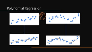
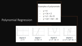
7. Underfitting and
Overfitting problems
• Underfitting looks a lot like not having studied enough for
an exam.
• Overfitting looks a lot like memorizing the entire textbook
instead of studying for the exam.
• How does that happen in machine learning?
• This is underfitting: our dataset is complex, and we
come to model it equipped with nothing but a simple
model.
• The model will not be able to capture the complexities of
the dataset.
• This is overfitting: our data is simple, but we try to fit
it to a model that is too complex. The model will be able
to fit our data, but it’ll memorize it instead of learning it.

8. Underfitting and
Overfitting problems
Which polynomial degree is suitable
for this data?
It is two
How Machines know that?!!
Let’s try degrees 1, 2, and 10

9. Underfitting and
Overfitting problems
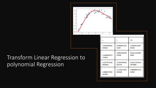
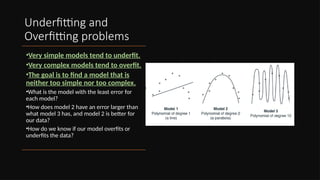
•Very simple models tend to underfit.
•Very complex models tend to overfit.
•The goal is to find a model that is
neither too simple nor too complex.
•What is the model with the least error for
each model?
•How does model 2 have an error larger than
what model 3 has, and model 2 is better for
our data?
•How do we know if our model overfits or
underfits the data?

10. Underfitting and Overfitting problems
[The Testing set solution]
•One way to determine if a model overfits
is by testing it, We divide the data into 2
sets
1.Training set (the majority)
2.Testing set
•We can know if there is an underfit or
overfit problem from train and test errors
and tune our hyperparamters based on
that.

11. Underfitting and
Overfitting problems
Models can
• Underfit: use a model that is too simple
for our dataset.
• Fit the data well: use a model that has
the right amount of complexity for our
dataset.
• Overfit: use a model that is too complex
for our dataset.
[Golden Rule]
•Never use testing data for training or to decide on the hyperparameters.
•We already broke this rule!
In the training set
• The underfit model will do poorly (large training
error).
• The good model will do well (small training
error).
• The overfit model will do very well (very small
training error).
In the testing set
• The underfit model will do poorly (large testing error).
• The good model will do well (small testing error).
• The overfit model will do poorly (large testing error).

12. Underfitting and Overfitting problems [The Validation set
solution]
We used our training data to train the three
models, and then we used the testing data
to decide which model to pick.
• Training set: for training all our models
• Validation set: for making decisions on
which model to use
• Testing set: for checking how well our
model did
This is called Simple (Holdout) Cross
Validation

13. Solving overfitting/underfitting problem [Model
Complexity Graph]
• A numerical way to decide how complex our model should
be and which model to use is to pick the one that has the
smallest validation error.
• One benefit of the model complexity graph is that no
matter how large our dataset is or how many different
models we try, it always looks like two curves: one that
always goes down (the training error) and one that goes
down and then back up (the validation error).
• In a large and complex dataset, these curves may oscillate,
and the behavior may be harder to spot.
• However, the model complexity graph is always a useful
tool for data scientists to find a good spot in this graph and
decide how complex their models should be to avoid both
underfitting and overfitting.

14. Solving overfitting/underfitting problem [Model Complexity]

15. Solving overfitting/underfitting problem [Early Stopping]
Which checkpoint should we pick for the same model?

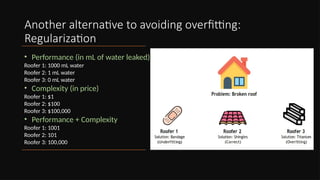
16. Another alternative to avoiding overfitting:
Regularization
• Performance (in mL of water leaked)
Roofer 1: 1000 mL water
Roofer 2: 1 mL water
Roofer 3: 0 mL water
• Complexity (in price)
Roofer 1: $1
Roofer 2: $100
Roofer 3: $100,000
• Performance + Complexity
Roofer 1: 1001
Roofer 2: 101
Roofer 3: 100,000

17. Another alternative to avoiding overfitting:
Regularization
• Now it is clear that Roofer 2 is the best one,
which means that optimizing performance and
complexity at the same time yields good results
that are also as simple as possible.
• In machine learning, what does represent the
performance cost and the complexity cost?
• This is what regularization is about: measuring
performance and complexity with two different
error functions and adding them to get a more
robust error function. This new error function
ensures that our model performs well and is not
very complex.
• In the following sections, we get into more detail
on how to define these two error functions.

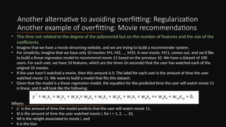
18. Another alternative to avoiding overfitting: Regularization
Another example of overfitting: Movie recommendations
• This time not related to the degree of the polynomial but on the number of features and the size of the
coefficients.
• Imagine that we have a movie streaming website, and we are trying to build a recommender system.
• For simplicity, imagine that we have only 10 movies: M1, M2, …, M10. A new movie, M11, comes out, and we’d like
to build a linear regression model to recommend movie 11 based on the previous 10. We have a dataset of 100
users. For each user, we have 10 features, which are the times (in seconds) that the user has watched each of the
original 10 movies.
• If the user hasn’t watched a movie, then this amount is 0. The label for each user is the amount of time the user
watched movie 11. We want to build a model that fits this dataset.
• Given that the model is a linear regression model, the equation for the predicted time the user will watch movie 11
is linear, and it will look like the following:
Where:
• yˆ is the amount of time the model predicts that the user will watch movie 11,
• Xi is the amount of time the user watched movie i, for i = 1, 2, …, 10,
• Wi is the weight associated to movie i, and
• b is the bias

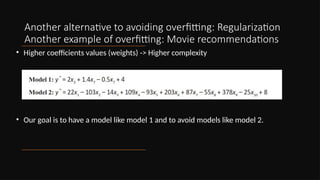
19. Another alternative to avoiding overfitting: Regularization
Another example of overfitting: Movie recommendations
• Higher coefficients values (weights) -> Higher complexity
• Our goal is to have a model like model 1 and to avoid models like model 2.

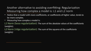
20. Another alternative to avoiding overfitting: Regularization
Measuring how complex a model is: L1 and L2 norm
• Notice that a model with more coefficients, or coefficients of higher value, tends to
be more complex.
• Measuring how complex a model is:
L1 Norm (lasso regularization): The sum of the absolute values of the coefficients
(weights).
L2 Norm (ridge regularization): The sum of the squares of the coefficients
(weights)

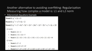
21. Another alternative to avoiding overfitting: Regularization
Measuring how complex a model is: L1 and L2 norm
• Polynomials Equations Example

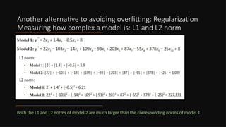
22. Another alternative to avoiding overfitting: Regularization
Measuring how complex a model is: L1 and L2 norm
Both the L1 and L2 norms of model 2 are much larger than the corresponding norms of model 1.

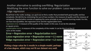
23. Another alternative to avoiding overfitting: Regularization
Modifying the error function to solve our problem: Lasso regression and
ridge regression
Recall that in the roofer analogy, our goal was to find a roofer that provided both good quality and low
complexity. We did this by minimizing the sum of two numbers: the measure of quality and the measure of
complexity. Regularization consists of applying the same principle to our machine learning model. For this,
we have two quantities: the regression error and the regularization term.
regression error: A measure of the quality of the model. In this case, it can be the absolute
or square errors.
regularization term: A measure of the complexity of the model. It can be the L1 or the L2
norm of the model.
Error = Regression error + Regularization term
Lasso regression error = Regression error + L1 norm
Ridge regression error = Regression error + L2 norm
Picking a large value for λ results in a simple model, perhaps
of a low degree, which may not fit our dataset very well.

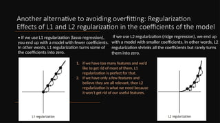
24. Another alternative to avoiding overfitting: Regularization
Effects of L1 and L2 regularization in the coefficients of the model
• If we use L1 regularization (lasso regression),
you end up with a model with fewer coefficients.
In other words, L1 regularization turns some of
the coefficients into zero.
If we use L2 regularization (ridge regression), we end up
with a model with smaller coefficients. In other words, L2
regularization shrinks all the coefficients but rarely turns
them into zero.
1. if we have too many features and we’d
like to get rid of most of them, L1
regularization is perfect for that.
2. If we have only a few features and
believe they are all relevant, then L2
regularization is what we need because
it won’t get rid of our useful features.

25. Regularization Example[Polynomial Features- Data Split]
“s7s/machine_learning_1/polynomial_regression/Polynomial_regression_regularization.ipynb”

26. Regularization Example[Without Regularization]
“s7s/machine_learning_1/polynomial_regression/Polynomial_regression_regularization.ipynb”

27. Regularization Example[Lasso Regularization]
“s7s/machine_learning_1/polynomial_regression/Polynomial_regression_regularization.ipynb”

28. Regularization Example[Ridge Regularization]
“s7s/machine_learning_1/polynomial_regression/Polynomial_regression_regularization.ipynb”

29. K-fold Cross Validation

30. Variance-Bias Tradeoff
https://towardsdatascience.com/understanding-the-bias-variance-tradeoff-165e6942b229