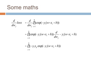
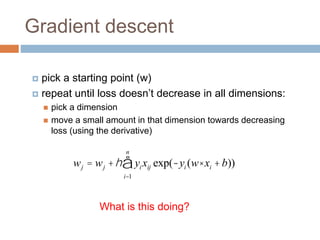
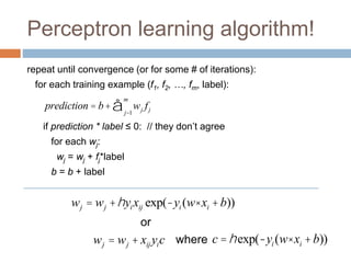
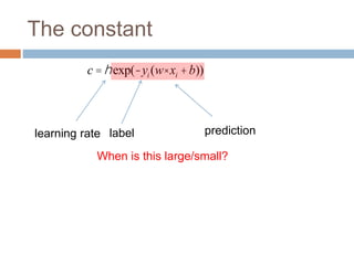
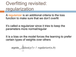
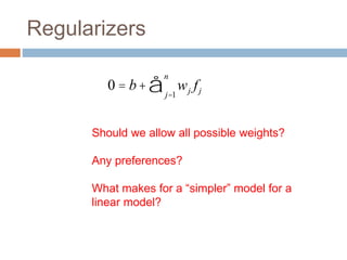
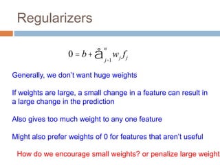
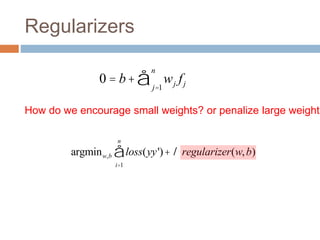
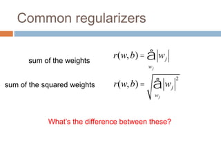
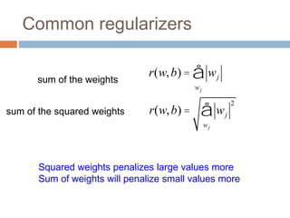
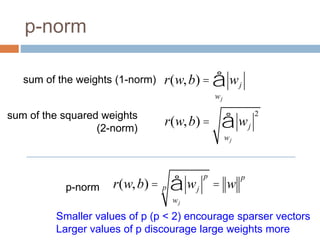
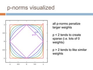
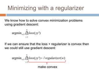
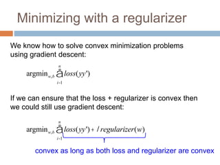
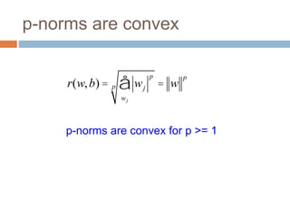
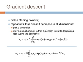
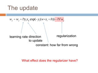
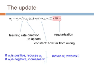
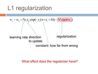
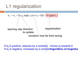
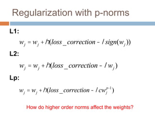
Regularization adds an additional term to the objective function being optimized in machine learning to prevent overfitting. Common regularizers include the L1 norm (sum of absolute weights), L2 norm (sum of squared weights), and Lp norms. The L1 norm encourages sparsity by driving small weights to exactly zero. Gradient descent can be used to minimize objective functions that combine a loss term and a regularizer, as long as the overall function remains convex. During gradient descent, the regularizer term pushes weights towards zero. Regularization is important for obtaining models that generalize well to new data.

1. REGULARIZATION
David Kauchak
CS 451 – Fall 2013

2. Admin
Assignment 5

3. Math so far…

4. Model-based machine learning
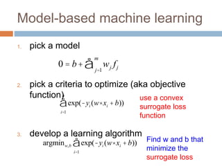
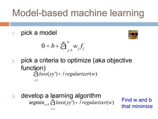
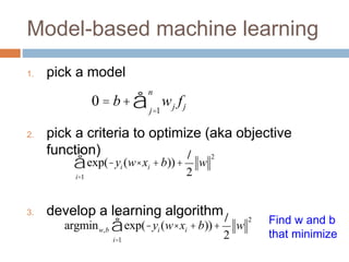
1. pick a model
2. pick a criteria to optimize (aka objective
function)
3. develop a learning algorithm
1 yi (w× xi +b) £ 0
[ ]
i=1
n
å
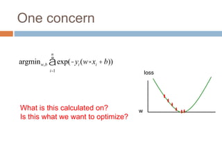
argminw,b 1 yi (w× xi +b) £ 0
[ ]
i=1
n
å Find w and b that
minimize the 0/1
loss
0 = b+ wj fj
j=1
m
å

5. Model-based machine learning
1. pick a model
2. pick a criteria to optimize (aka objective
function)
3. develop a learning algorithm
exp(-yi (w× xi +b))
i=1
n
å
argminw,b exp(-yi (w× xi +b))
i=1
n
å Find w and b that
minimize the
surrogate loss
use a convex
surrogate loss
function
0 = b+ wj fj
j=1
m
å

6. Finding the minimum
You’re blindfolded, but you can see out of the bottom of
the blindfold to the ground right by your feet. I drop you
off somewhere and tell you that you’re in a convex shaped
valley and escape is at the bottom/minimum. How do you

7. Gradient descent
 pick a starting point (w)
 repeat until loss doesn’t decrease in all dimensions:
 pick a dimension
 move a small amount in that dimension towards decreasing
loss (using the derivative)
wj = wj -h
d
dwj
loss(w)

8. Some maths
=
d
dwj
exp(-yi (w× xi +b))
i=1
n
å
d
dwj
loss
= exp(-yi (w× xi +b))
d
dwj
i=1
n
å - yi (w× xi +b)
= -yi xij exp(-yi (w× xi +b))
i=1
n
å

9. Gradient descent
 pick a starting point (w)
 repeat until loss doesn’t decrease in all dimensions:
 pick a dimension
 move a small amount in that dimension towards decreasing
loss (using the derivative)
wj = wj +h yi xij exp(-yi (w× xi +b))
i=1
n
å
What is this doing?

10. Perceptron learning algorithm!
repeat until convergence (or for some # of iterations):
for each training example (f1, f2, …, fm, label):
if prediction * label ≤ 0: // they don’t agree
for each wj:
wj = wj + fj*label
b = b + label
prediction = b+ wj fj
j=1
m
å
wj = wj +hyixij exp(-yi (w× xi +b))
wj = wj + xij yic
or
where c =hexp(-yi (w× xi +b))

11. The constant
c =hexp(-yi (w× xi +b))
When is this large/small?
prediction
label
learning rate

12. The constant
c =hexp(-yi (w× xi +b))
prediction
label
If they’re the same sign, as the
predicted gets larger there
update gets smaller
If they’re different, the more
different they are, the bigger the
update

13. One concern
What is this calculated on?
Is this what we want to optimize?
argminw,b exp(-yi (w× xi +b))
i=1
n
å
w
loss

14. Perceptron learning algorithm!
repeat until convergence (or for some # of iterations):
for each training example (f1, f2, …, fm, label):
if prediction * label ≤ 0: // they don’t agree
for each wj:
wj = wj + fj*label
b = b + label
prediction = b+ wj fj
j=1
m
å
wj = wj +hyixij exp(-yi (w× xi +b))
wj = wj + xij yic
or
where c =hexp(-yi (w× xi +b))
Note: for gradient descent, we always update

15. One concern
w
loss
argminw,b exp(-yi (w× xi +b))
i=1
n
å
We’re calculating this on the
training set
We still need to be careful about
overfitting!
The min w,b on the training set is
generally NOT the min for the test
set How did we deal with this for the perceptron algorithm?

16. Overfitting revisited:
regularization
A regularizer is an additional criteria to the loss
function to make sure that we don’t overfit
It’s called a regularizer since it tries to keep the
parameters more normal/regular
It is a bias on the model forces the learning to prefer
certain types of weights over others
argminw,b loss(yy')+l regularizer(w,b)
i=1
n
å

17. Regularizers
0 = b+ wj fj
j=1
n
å
Should we allow all possible weights?
Any preferences?
What makes for a “simpler” model for a
linear model?

18. Regularizers
Generally, we don’t want huge weights
If weights are large, a small change in a feature can result in
a large change in the prediction
Also gives too much weight to any one feature
Might also prefer weights of 0 for features that aren’t useful
How do we encourage small weights? or penalize large weights
0 = b+ wj fj
j=1
n
å

19. Regularizers
How do we encourage small weights? or penalize large weights
argminw,b loss(yy')+l regularizer(w,b)
i=1
n
å
0 = b+ wj fj
j=1
n
å

20. Common regularizers
What’s the difference between these?
r(w,b) = wj
wj
å
sum of the weights
sum of the squared weights r(w,b) = wj
2
wj
å

21. Common regularizers
Squared weights penalizes large values more
Sum of weights will penalize small values more
sum of the weights
sum of the squared weights
r(w,b) = wj
wj
å
r(w,b) = wj
2
wj
å

22. p-norm
sum of the weights (1-norm)
sum of the squared weights
(2-norm)
p-norm r(w,b) = wj
p
wj
å
p = w
p
Smaller values of p (p < 2) encourage sparser vectors
Larger values of p discourage large weights more
r(w,b) = wj
wj
å
r(w,b) = wj
2
wj
å

23. p-norms visualized
w1
w2
lines indicate penalty = 1
For example, if w1 = 0.5
p w2
1 0.5
1.5 0.75
2 0.87
3 0.95
∞ 1

24. p-norms visualized
all p-norms penalize
larger weights
p < 2 tends to create
sparse (i.e. lots of 0
weights)
p > 2 tends to like similar
weights

25. Model-based machine learning
1. pick a model
2. pick a criteria to optimize (aka objective
function)
3. develop a learning algorithm
0 = b+ wj fj
j=1
n
å
loss(yy')
i=1
n
å + lregularizer(w)
argminw,b loss(yy')
i=1
n
å + lregularizer(w) Find w and b
that minimize

26. Minimizing with a regularizer
argminw,b loss(yy')
i=1
n
å +lregularizer(w)
argminw,b loss(yy')
i=1
n
å
We know how to solve convex minimization problems
using gradient descent:
If we can ensure that the loss + regularizer is convex then
we could still use gradient descent:
make convex

27. Convexity revisited
One definition: The line segment between
any two points on the function is above the
function
Mathematically, f is convex if for all x1, x2:
f (tx1 +(1-t)x2 )£ tf (x1)+(1-t)f (x2 ) " 0 < t <1
the value of the
function at some
point between x1 and
x2
the value at some
point on the line
segment between
x1 and x2

28. Adding convex functions
Claim: If f and g are convex functions then so is
the function z=f+g
f (tx1 +(1-t)x2 )£ tf (x1)+(1-t)f (x2 ) " 0 < t <1
Mathematically, f is convex if for all x1, x2:
Prove:
z(tx1 +(1-t)x2 )£ tz(x1)+(1-t)z(x2 ) " 0 < t <1

29. Adding convex functions
z(tx1 +(1-t)x2 )= f (tx1 +(1-t)x2 )+g(tx1 +(1-t)x2 )
tz(x1)+(1-t)z(x2 )= tf (x1)+tg(x1)+(1-t)f (x2 )+(1-t)g(x2 )
= tf (x1)+(1-t)f (x2 )+tg(x1)+(1-t)g(x2 )
f (tx1 +(1-t)x2 )£ tf (x1)+(1-t)f (x2 )
g(tx1 +(1-t)x2 )£ tg(x1)+(1-t)g(x2 )
Then, given that:
By definition of the sum of two functions:
We know:
f (tx1 +(1-t)x2 )+g(tx1 +(1-t)x2 )£ tf (x1)+(1-t)f (x2 )+tg(x1)+(1-t)g(x2 )
z(tx1 +(1-t)x2 ) £ tz(x1)+(1-t)z(x2 )
So:

30. Minimizing with a regularizer
argminw,b loss(yy')
i=1
n
å +lregularizer(w)
argminw,b loss(yy')
i=1
n
å
We know how to solve convex minimization problems
using gradient descent:
If we can ensure that the loss + regularizer is convex then
we could still use gradient descent:
convex as long as both loss and regularizer are convex

31. p-norms are convex
r(w,b) = wj
p
wj
å
p = w
p
p-norms are convex for p >= 1

32. Model-based machine learning
1. pick a model
2. pick a criteria to optimize (aka objective
function)
3. develop a learning algorithm
0 = b+ wj fj
j=1
n
å
exp(-yi (w× xi +b))
i=1
n
å +
l
2
w
2
argminw,b exp(-yi (w× xi +b))
i=1
n
å +
l
2
w
2 Find w and b
that minimize

33. Our optimization criterion
argminw,b exp(-yi (w× xi +b))
i=1
n
å +
l
2
w
2
Loss function: penalizes
examples where the
prediction is different than
the label
Regularizer: penalizes large
weights
Key: this function is convex allowing us to use gradient des

34. Gradient descent
 pick a starting point (w)
 repeat until loss doesn’t decrease in all dimensions:
 pick a dimension
 move a small amount in that dimension towards decreasing
loss (using the derivative)
wi = wi -h
d
dwi
(loss(w)+regularizer(w,b))
argminw,b exp(-yi (w× xi +b))
i=1
n
å +
l
2
w
2

35. Some more maths
d
dwj
exp(-yi (w× xi +b))
i=1
n
å +
l
2
w
2
d
dwj
objective =
= - yixij exp(-yi (w× xi +b))
i=1
n
å +lwj
…
(some math happens)

36. Gradient descent
 pick a starting point (w)
 repeat until loss doesn’t decrease in all dimensions:
 pick a dimension
 move a small amount in that dimension towards decreasing
loss (using the derivative)
wj = wj +h yi xij exp(-yi (w× xi +b))
i=1
n
å -hlwj
wi = wi -h
d
dwi
(loss(w)+regularizer(w,b))

37. The update
wj = wj +hyixij exp(-yi (w× xi +b))-hlwj
regularization
direction
to update
learning rate
constant: how far from wrong
What effect does the regularizer have?

38. The update
If wj is positive, reduces wj
If wj is negative, increases wj
moves wj towards 0
wj = wj +hyixij exp(-yi (w× xi +b))-hlwj
regularization
direction
to update
learning rate
constant: how far from wrong

39. L1 regularization
argminw,b exp(-yi (w× xi +b))
i=1
n
å + w
d
dwj
exp(-yi (w× xi +b))
i=1
n
å + l w
d
dwj
objective =
= - yixij exp(-yi (w× xi +b))
i=1
n
å +lsign(wj )

40. L1 regularization
wj = wj +hyixij exp(-yi (w× xi +b))-hlsign(wj )
regularization
direction
to update
learning rate
constant: how far from wrong
What effect does the regularizer have?

41. L1 regularization
wj = wj +hyixij exp(-yi (w× xi +b))-hlsign(wj )
regularization
direction
to update
learning rate
constant: how far from wrong
If wj is positive, reduces by a constant
If wj is negative, increases by a constant
moves wj towards 0
regardless of magnitud

42. Regularization with p-norms
L1:
L2:
Lp:
wj = wj +h(loss_correction-lsign(wj ))
wj = wj +h(loss_correction-lwj )
wj = wj +h(loss_correction-lcwj
p-1
)
How do higher order norms affect the weights?

43. Regularizers summarized
L1 is popular because it tends to result in sparse
solutions (i.e. lots of zero weights)
However, it is not differentiable, so it only works for
gradient descent solvers
L2 is also popular because for some loss functions,
it can be solved directly (no gradient descent
required, though often iterative solvers still)
Lp is less popular since they don’t tend to shrink the
weights enough

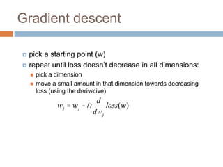
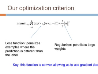
44. The other loss functions
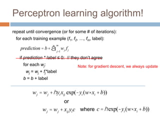
wj = wj +hyixijc
Without regularization, the generic update is:
where
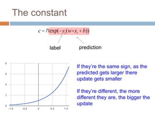
c = exp(-yi (w× xi +b))
c =1[yy' <1]
exponential
hinge loss
squared error
wj = wj +h(yi -(w× xi +b)xij )

45. Many tools support these different
combinations
Look at scikit learning package:
http://scikit-learn.org/stable/modules/sgd.html

46. Common names
(Ordinary) Least squares: squared loss
Ridge regression: squared loss with L2
regularization
Lasso regression: squared loss with L1
regularization
Elastic regression: squared loss with L1 AND L2
regularization
Logistic regression: logistic loss

47. Real results