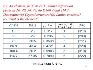
Download to read offline


![ACTUAL EXAMPLE: PYRITE THIN FILM
FeS2 – cubic (a = 5.43 Å)
Random crystal orientations
On casual inspection, peaks give us d-spacings, unit cell size, crystal
symmetry, preferred orientation, crystal size, and impurity phases (none!)
111
200
210
211
220
311
Cu Kα = 1.54 Å
2 Theta
Intensity
“powder pattern”
2θ = 28.3° → d = 1.54/[2sin(14.15)]
= 3.13 Å = d111
reference pattern from ICDD
(1,004,568+ datasets)](https://image.slidesharecdn.com/2634-230204053651-e928014b/85/263-4-pdf-25-320.jpg)


![Brillouin Zone of Diamond and
Zincblende Structure (FCC Lattice)
• Notation:
– Zone Edge or
surface : Roman
alphabet
– Interior of Zone:
Greek alphabet
– Center of Zone or
origin: G
3D BAND STRUCTURE
Notation:
D<=>[100]
direction
X<=>BZ edge
along [100]
direction
L<=>[111]
direction
L<=>BZ edge
along [111]
direction273](https://image.slidesharecdn.com/2634-230204053651-e928014b/85/263-4-pdf-55-320.jpg)


![Φ = 4(fNa + fCl) when h, k, l, all even
Φ = 4(fNa - fCl) when h, k, l all odd
Φ = 0 otherwise
( )
,
[ ][ ]
i h k l
Na Cl FCC
f f e S
K K
306
( ) ( ) ( ) ( )
[ ][1 ]
i h k l i h k i h l i l k
Na Cl
f f e e e e
K](https://image.slidesharecdn.com/2634-230204053651-e928014b/85/263-4-pdf-88-320.jpg)


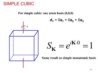
![DIAMOND STRUCTURE
Diamond: FCC lattice with two-atom basis (0,0,0,), (¼,¼,¼)
( )
0 4
, ,
( /2)( )
,
[ ][ ]
[1 ][ ]
a
iK x y z
iK
diamond FCC
i h k l
FCC
S e e S
e S
K K
K
S = 8 h + k + l twice an even number
S = 4(1 ± i) h + k + l odd
S = 0 h + k + l twice an odd number
IFCC : all nonvanishing spots have equal intensity.
Idiamond : spots allowed by FCC have relative intensities
of 64, 32, or 0. 309
Only for all even or all odd hkl is S ≠ 0. For these unmixed values,
Additional condition:](https://image.slidesharecdn.com/2634-230204053651-e928014b/85/263-4-pdf-91-320.jpg)


![352
k-SPACE GEOMETRY
for rotation around [001]
of cubic crystal:
monitor {011}: expect 4 peaks separated by 90° rotation.
monitor {111}: expect 4 peaks separated by 90° rotation.
(ignoring possible systematic absences)
two examples:](https://image.slidesharecdn.com/2634-230204053651-e928014b/85/263-4-pdf-134-320.jpg)
![PHI SCAN EXAMPLE
1 um GaN (wurtzite) on Silicon(111)
2-theta scan proves
uni-axial texture phi scan proves
bi-axial texture (epitaxy)
(002)
(1011)
In plane alignment: GaN[1120]//Si[110] 353](https://image.slidesharecdn.com/2634-230204053651-e928014b/85/263-4-pdf-135-320.jpg)


![Why ED patterns have so many spots
λX-ray = hc/E = 0.154 nm @ 8 keV
λe- = h/[2m0eV(1 + eV/2m0c2)]1/2 = 0.0037 nm @ 100 keV
Typically, in X-ray or neutron diffraction only one reciprocal lattice point
is on the surface of the Ewald sphere at one time.
In electron diffraction the Ewald sphere is not highly curved b/c of the
very short wavelength electrons that are used. This nearly-flat Ewald
sphere intersects with many reciprocal lattice points at once.
- In real crystals reciprocal lattice points are not infinitely small and in a
real microscope the Ewald sphere is not infinitely thin
368](https://image.slidesharecdn.com/2634-230204053651-e928014b/85/263-4-pdf-150-320.jpg)


This document discusses various techniques for crystal structure analysis using diffraction of x-rays, electrons, and neutrons. It begins by introducing Bragg diffraction and references several textbooks on topics like x-ray diffraction, small-angle scattering, and protein crystallography. The document then covers the fundamentals of elastic and inelastic scattering, Bragg's law of diffraction, diffraction orders, and applications of techniques like powder diffraction, single-crystal diffraction, and thin film analysis.


