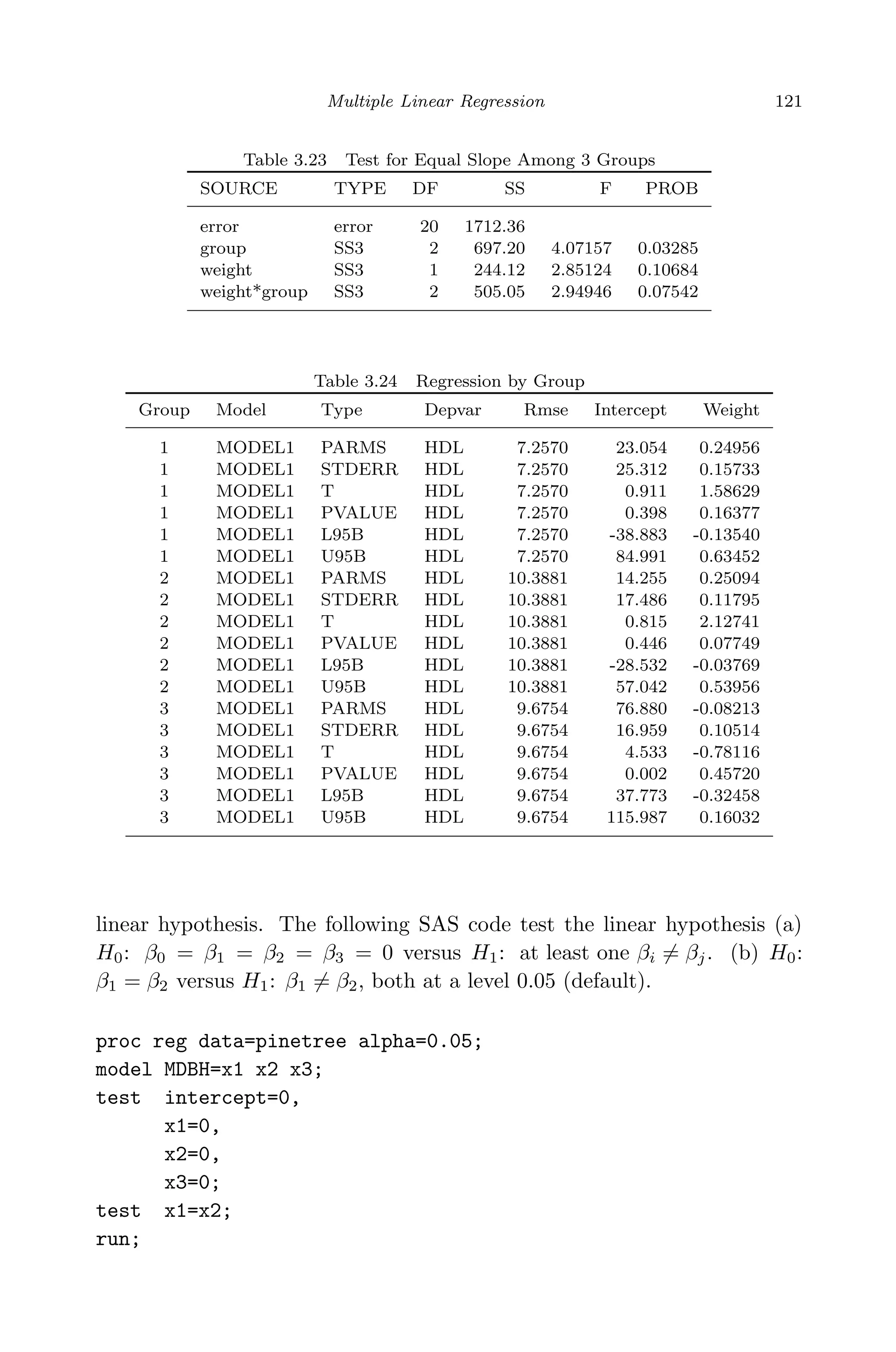
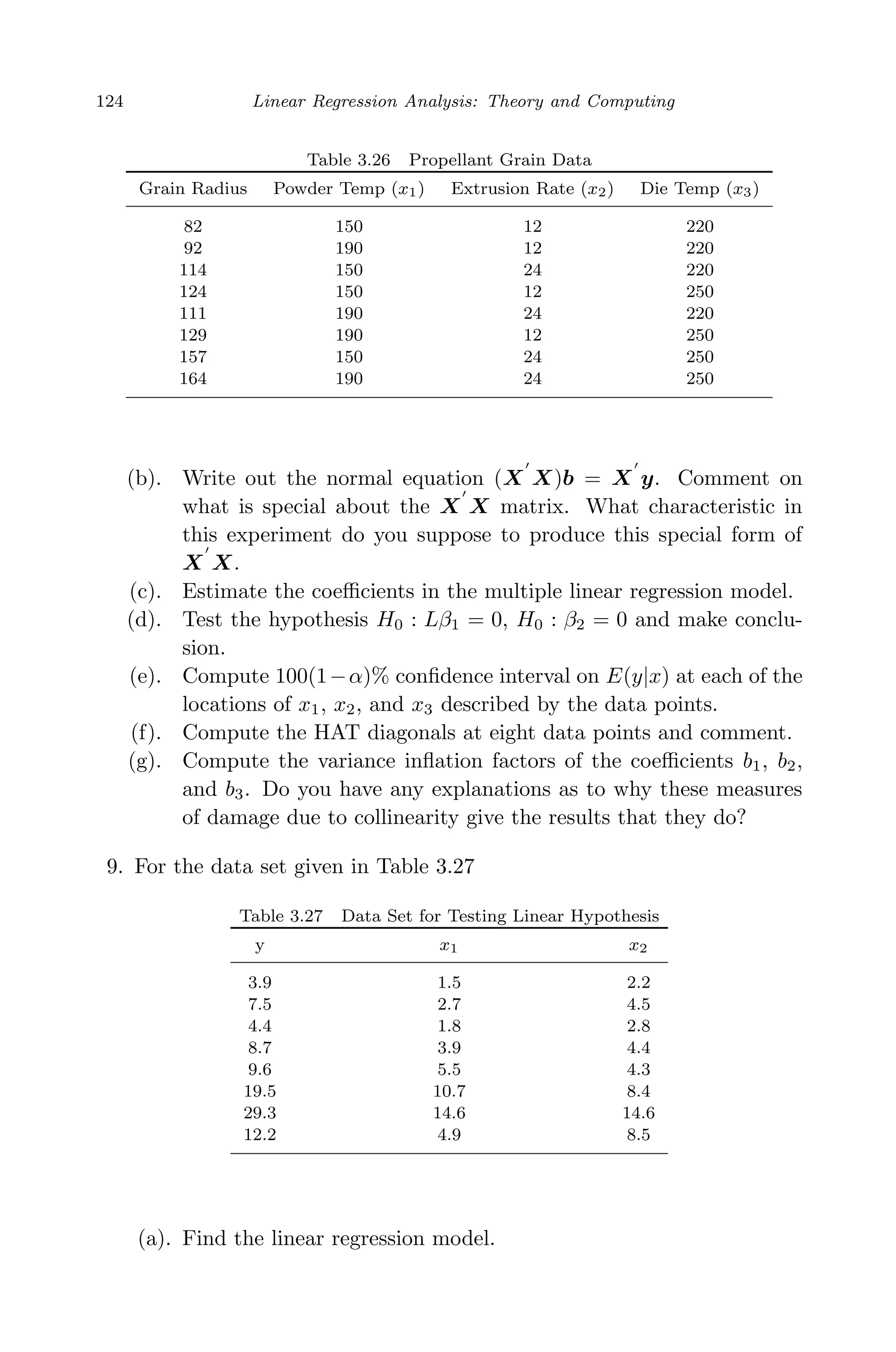
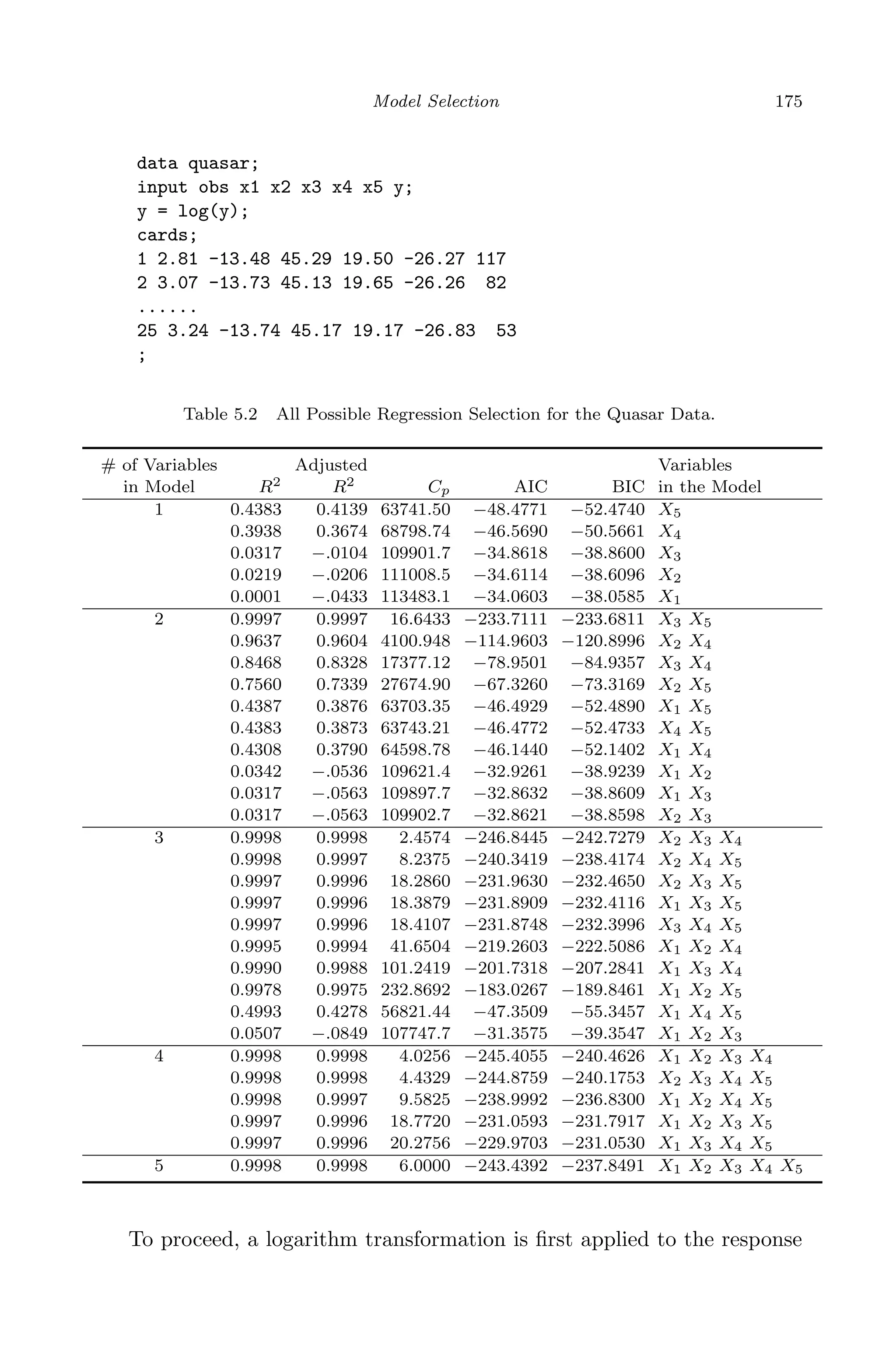
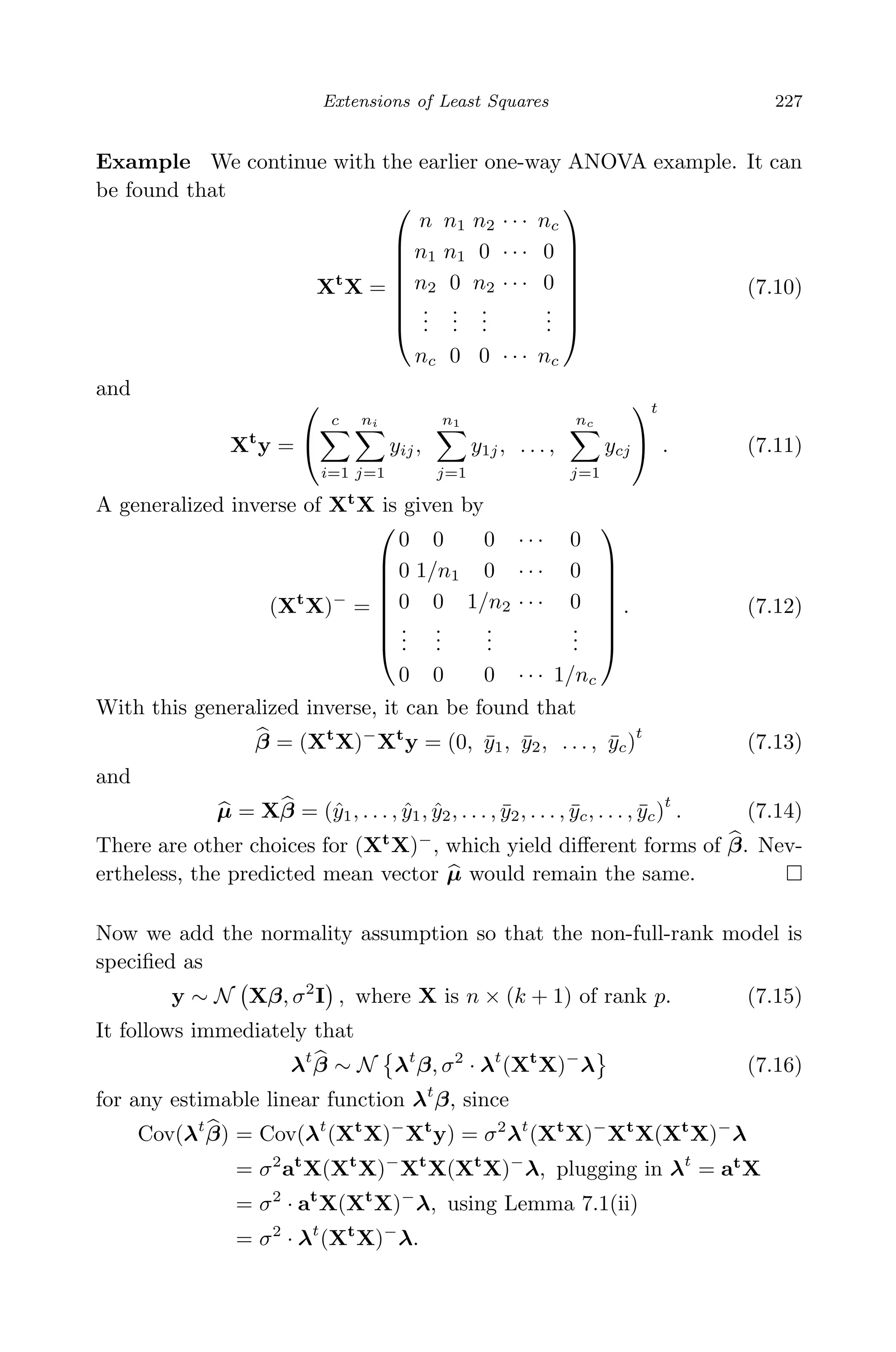
Downloaded 121 times


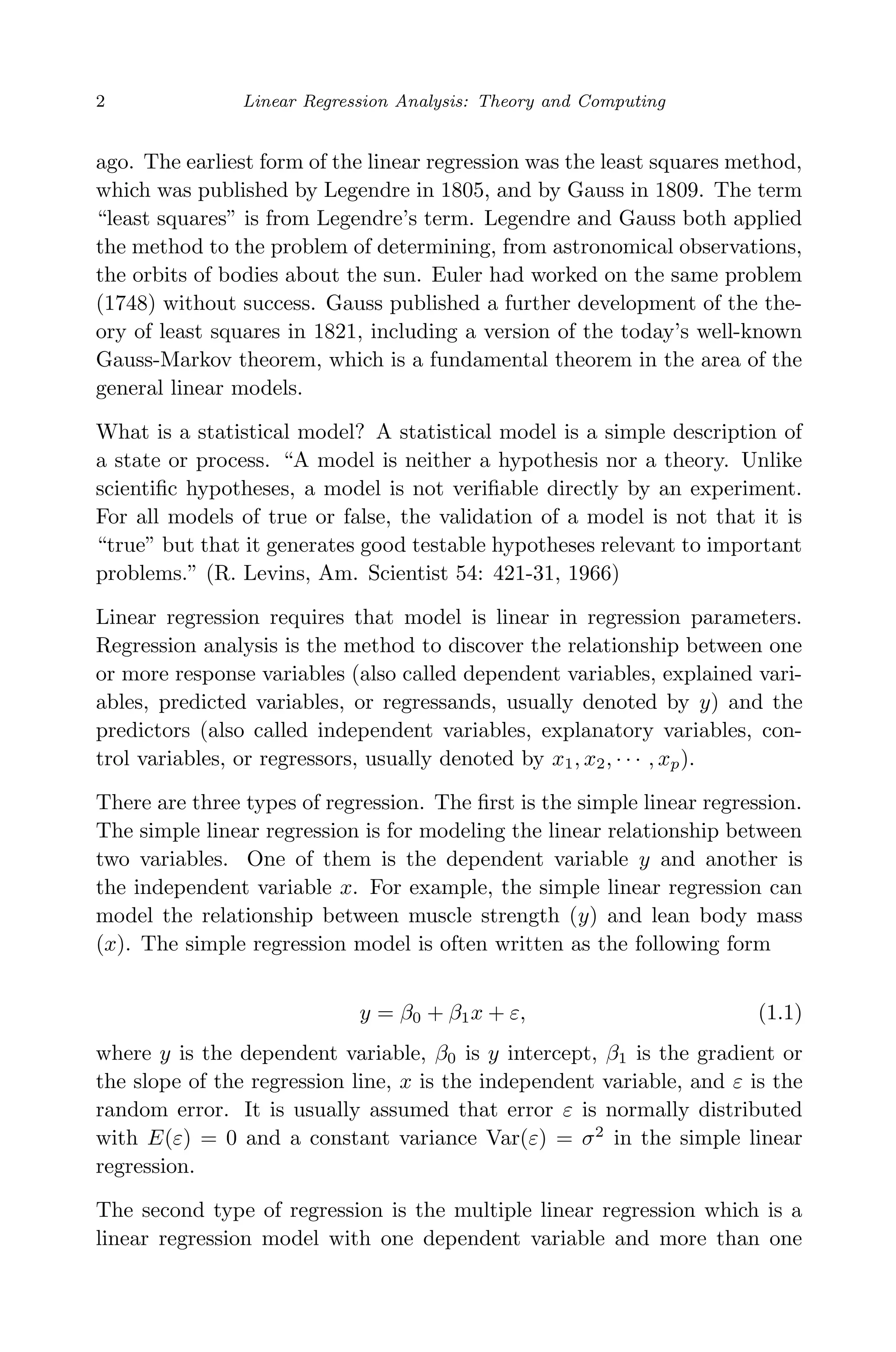


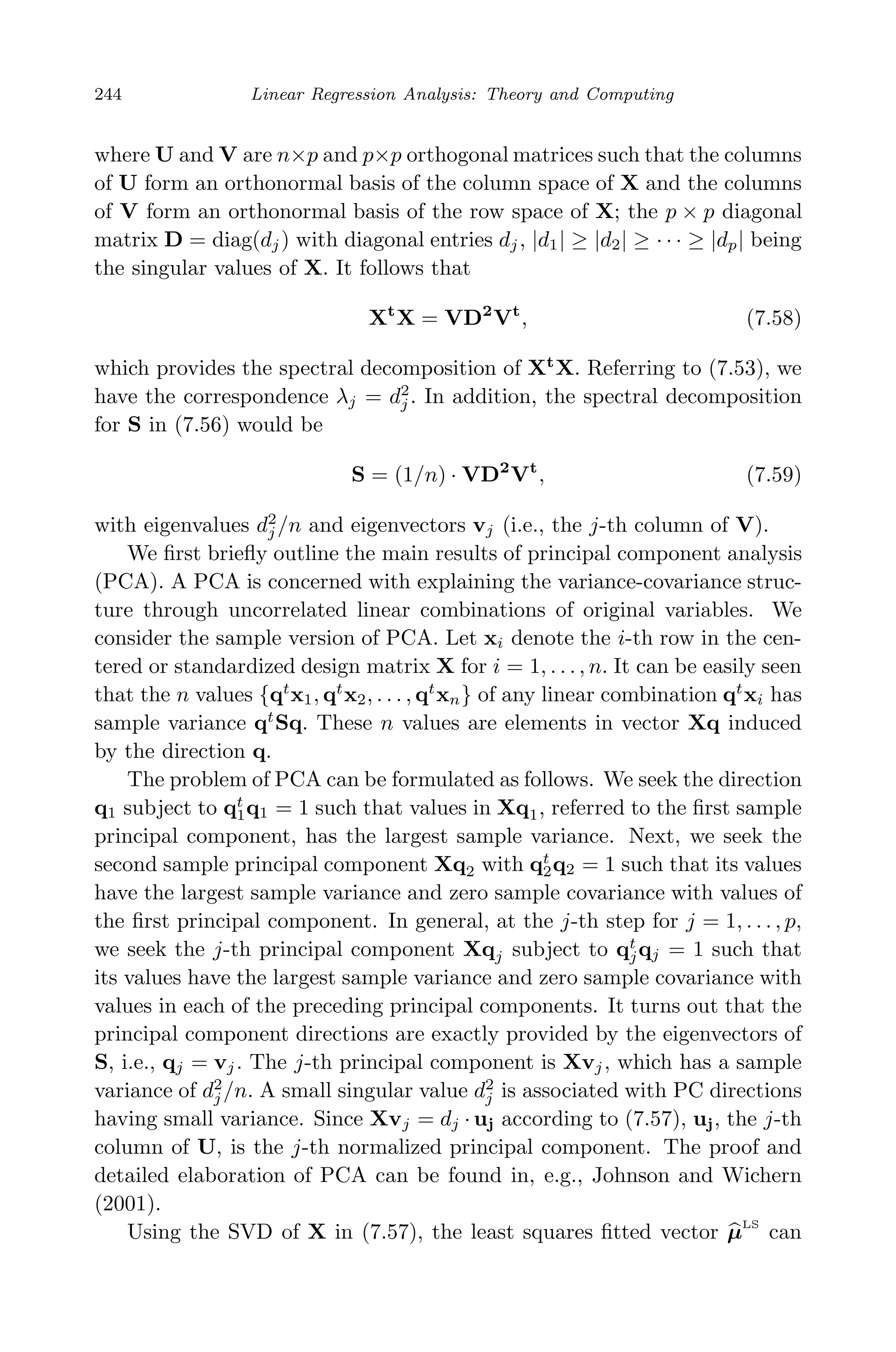
![April 29, 2009 11:50 World Scientific Book - 9in x 6in Regression˙master
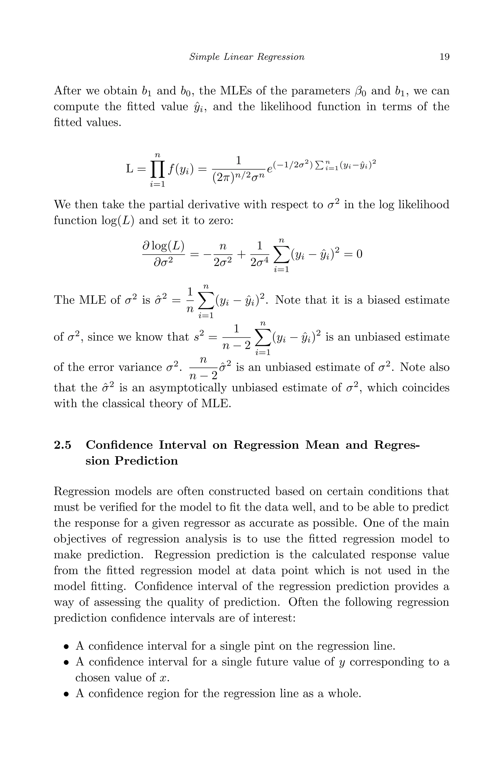
10 Linear Regression Analysis: Theory and Computing
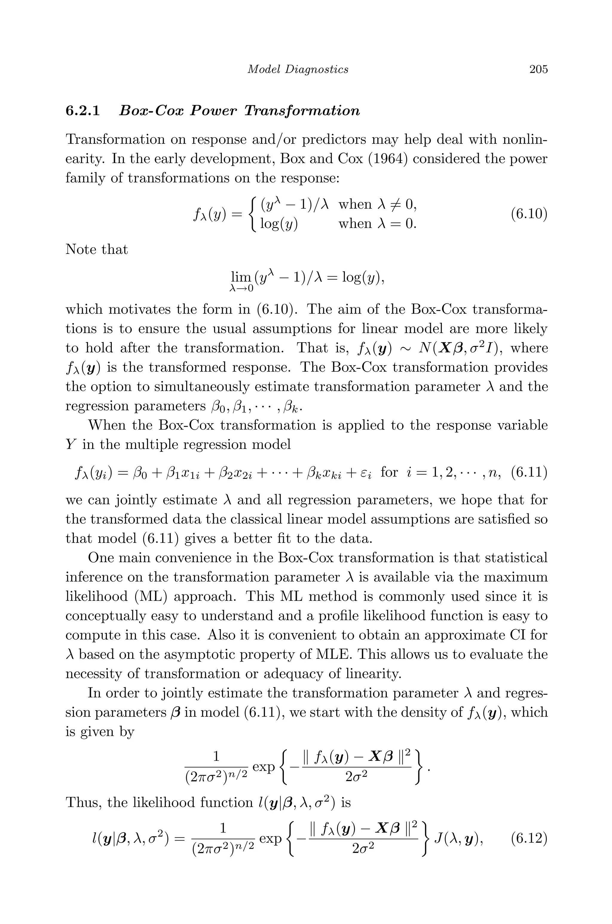
random error. The dependent variable is also called response variable, and
the independent variable is called explanatory or predictor variable. An
explanatory variable explains causal changes in the response variables. A
more general presentation of a regression model may be written as
y = E(y) + ,
where E(y) is the mathematical expectation of the response variable. When
E(y) is a linear combination of exploratory variables x1, x2, · · · , xk the
regression is the linear regression. If k = 1 the regression is the simple linear
regression. If E(y) is a nonlinear function of x1, x2, · · · , xk the regression
is nonlinear. The classical assumptions on error term are E(ε) = 0 and a
constant variance Var(ε) = σ2
. The typical experiment for the simple linear
regression is that we observe n pairs of data (x1, y1), (x2, y2), · · · , (xn, yn)
from a scientific experiment, and model in terms of the n pairs of the data
can be written as
yi = β0 + β1xi + εi for i = 1, 2, · · · , n,
with E(εi) = 0, a constant variance Var(εi) = σ2
, and all εi’s are indepen-
dent. Note that the actual value of σ2
is usually unknown. The values of
xi’s are measured “exactly”, with no measurement error involved. After
model is specified and data are collected, the next step is to find “good”
estimates of β0 and β1 for the simple linear regression model that can best
describe the data came from a scientific experiment. We will derive these
estimates and discuss their statistical properties in the next section.
2.2 Least Squares Estimation
The least squares principle for the simple linear regression model is to
find the estimates b0 and b1 such that the sum of the squared distance
from actual response yi and predicted response ˆyi = β0 + β1xi reaches the
minimum among all possible choices of regression coefficients β0 and β1.
i.e.,
(b0, b1) = arg min
(β0,β1)
n
i=1
[yi − (β0 + β1xi)]2
.
The motivation behind the least squares method is to find parameter es-
timates by choosing the regression line that is the most “closest” line to](https://image.slidesharecdn.com/xinyanxiaogangsulinearregressionanalysisbookfi-140714092751-phpapp02/75/Xin-yan-xiao_gang_su-_linear_regression_analysis-book_fi-org-31-2048.jpg)
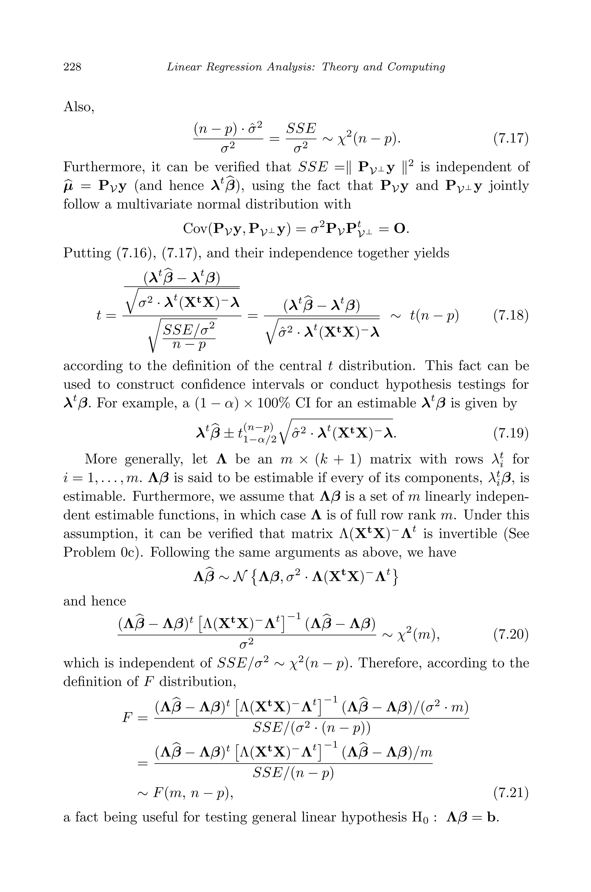
![April 29, 2009 11:50 World Scientific Book - 9in x 6in Regression˙master
Simple Linear Regression 11
all data points (xi, yi). Mathematically, the least squares estimates of the
simple linear regression are given by solving the following system:
∂
∂β0
n
i=1
[yi − (β0 + β1xi)]2
= 0 (2.1)
∂
∂β1
n
i=1
[yi − (β0 + β1xi)]2
= 0 (2.2)
Suppose that b0 and b1 are the solutions of the above system, we can de-
scribe the relationship between x and y by the regression line ˆy = b0 + b1x
which is called the fitted regression line by convention. It is more convenient
to solve for b0 and b1 using the centralized linear model:
yi = β∗
0 + β1(xi − ¯x) + εi,
where β0 = β∗
0 − β1 ¯x. We need to solve for
∂
∂β∗
0
n
i=1
[yi − (β∗
0 + β1(xi − ¯x))]2
= 0
∂
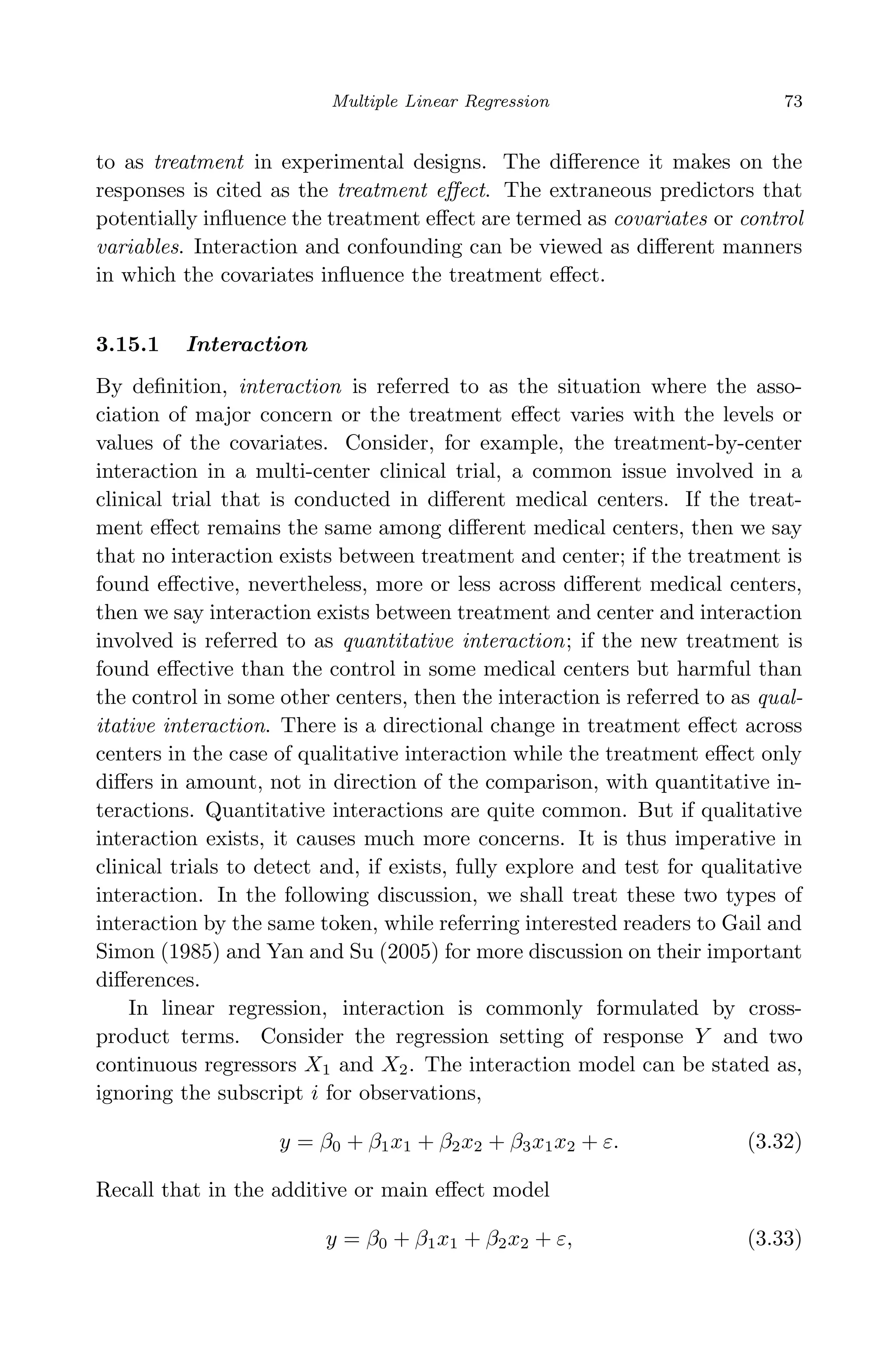
∂β1
n
i=1
[yi − (β∗
0 + β1(xi − ¯x))]2
= 0
Taking the partial derivatives with respect to β0 and β1 we have
n
i=1
[yi − (β∗
0 + β1(xi − ¯x))] = 0
n
i=1
[yi − (β∗
0 + β1(xi − ¯x))](xi − ¯x) = 0
Note that
n
i=1
yi = nβ∗
0 +
n
i=1
β1(xi − ¯x) = nβ∗
0 (2.3)
Therefore, we have β∗
0 =
1
n
n
i=1
yi = ¯y. Substituting β∗
0 by ¯y in (2.3) we
obtain
n
i=1
[yi − (¯y + β1(xi − ¯x))](xi − ¯x) = 0.](https://image.slidesharecdn.com/xinyanxiaogangsulinearregressionanalysisbookfi-140714092751-phpapp02/75/Xin-yan-xiao_gang_su-_linear_regression_analysis-book_fi-org-32-2048.jpg)
![April 29, 2009 11:50 World Scientific Book - 9in x 6in Regression˙master
14 Linear Regression Analysis: Theory and Computing
Theorem 2.3. Var(b1) =
σ2
nSxx
.
Proof.
Var(b1) = Var
Sxy
Sxx
=
1
S2
xx
Var
1
n
n
i=1
(yi − ¯y)(xi − ¯x)
=
1
S2
xx
Var
1
n
n
i=1
yi(xi − ¯x)
=
1
S2
xx
1
n2
n
i=1
(xi − ¯x)2
Var(yi)
=
1
S2
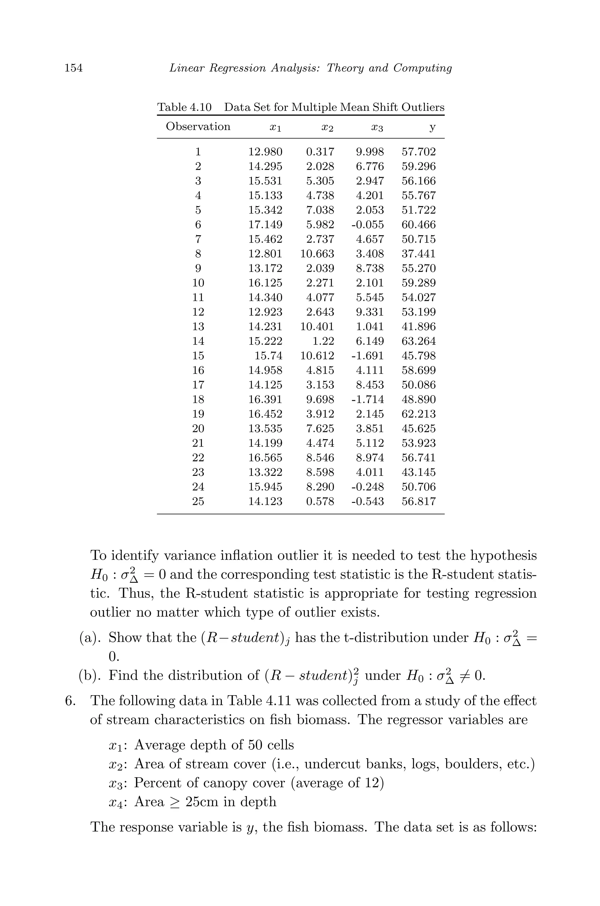
xx
1
n2
n
i=1
(xi − ¯x)2
σ2
=
σ2
nSxx
Theorem 2.4. The least squares estimator b1 and ¯y are uncorrelated. Un-
der the normality assumption of yi for i = 1, 2, · · · , n, b1 and ¯y are normally
distributed and independent.
Proof.
Cov(b1, ¯y) = Cov(
Sxy
Sxx
, ¯y)
=
1
Sxx
Cov(Sxy, ¯y)
=
1
nSxx
Cov
n
i=1
(xi − ¯x)(yi − ¯y), ¯y
=
1
nSxx
Cov
n
i=1
(xi − ¯x)yi, ¯y
=
1
n2Sxx
Cov
n
i=1
(xi − ¯x)yi,
n
i=1
yi
=
1
n2Sxx
n
i,j=1
(xi − ¯x) Cov(yi, yj)
Note that Eεi = 0 and εi’s are independent we can write
Cov(yi, yj) = E[ (yi − Eyi)(yj − Eyj) ] = E(εi, εj) =
σ2
, if i = j
0, if i = j](https://image.slidesharecdn.com/xinyanxiaogangsulinearregressionanalysisbookfi-140714092751-phpapp02/75/Xin-yan-xiao_gang_su-_linear_regression_analysis-book_fi-org-35-2048.jpg)
![April 29, 2009 11:50 World Scientific Book - 9in x 6in Regression˙master
16 Linear Regression Analysis: Theory and Computing
linear regression model. We will see in later chapters that it is true for all
general linear models. In particular, in a multiple linear regression model
with p parameters the denominator should be n − p in order to construct
an unbiased estimator of the error variance σ2
. Detailed discussion can be
found in later chapters. The unbiasness of estimator s2
for the simple linear
regression can be shown in the following derivations.
yi − ˆyi = yi − b0 − b1xi = yi − (¯y − b1 ¯x) − b1xi = (yi − ¯y) − b1(xi − ¯x)
It follows that
n
i=1
(yi − ˆyi) =
n
i=1
(yi − ¯y) − b1
n
i=1
(xi − ¯x) = 0.
Note that (yi − ˆyi)xi = [(yi − ¯y) − b1(xi − ¯x)]xi, hence we have
n
i=1
(yi − ˆyi)xi =
n
i=1
[(yi − ¯y) − b1(xi − ¯x)]xi
=
n
i=1
[(yi − ¯y) − b1(xi − ¯x)](xi − ¯x)
=
n
i=1
(yi − ¯y)(xi − ¯x) − b1
n
i=1
(xi − ¯x)2
= n(Sxy − b1Sxx) = n Sxy −
Sxy
Sxx
Sxx = 0
To show that s2
is an unbiased estimate of the error variance, first we note
that
(yi − ˆyi)2
= [(yi − ¯y) − b1(xi − ¯x)]2
,
therefore,
n
i=1
(yi − ˆyi)2
=
n
i=1
[(yi − ¯y) − b1(xi − ¯x)]2
=
n
i=1
(yi − ¯y)2
− 2b1
n
i=1
(xi − ¯x)(yi − ¯yi) + b2
1
n
i=1
(xi − ¯x)2
=
n
i=1
(yi − ¯y)2
− 2nb1Sxy + nb2
1Sxx
=
n
i=1
(yi − ¯y)2
− 2n
Sxy
Sxx
Sxy + n
S2
xy
S2
xx
Sxx
=
n
i=1
(yi − ¯y)2
− n
S2
xy
Sxx](https://image.slidesharecdn.com/xinyanxiaogangsulinearregressionanalysisbookfi-140714092751-phpapp02/75/Xin-yan-xiao_gang_su-_linear_regression_analysis-book_fi-org-37-2048.jpg)
![April 29, 2009 11:50 World Scientific Book - 9in x 6in Regression˙master
Simple Linear Regression 17
Since
(yi − ¯y)2
= [β1(xi − ¯x) + (εi − ¯ε)]2
and
(yi − ¯y)2
= β2
1(xi − ¯x)2
+ (εi − ¯ε)2
+ 2β1(xi − ¯x)(εi − ¯ε),
therefore,
E(yi − ¯y)2
= β2
1(xi − ¯x)2
+ E(εi − ¯ε)2
= β2
1(xi − ¯x)2
+
n − 1
n
σ2
,
and
n
i=1
E(yi − ¯y)2
= nβ2
1Sxx +
n
i=1
n − 1
n
σ2
= nβ2
1Sxx + (n − 1)σ2
.
Furthermore, we have
E(Sxy) = E
1
n
n
i=1
(xi − ¯x)(yi − ¯y)
=
1
n
E
n
i=1
(xi − ¯x)yi
=
1
n
n
i=1
(xi − ¯x)Eyi
=
1
n
n
i=1
(xi − ¯x)(β0 + β1xi)
=
1
n
β1
n
i=1
(xi − ¯x)xi
=
1
n
β1
n
i=1
(xi − ¯x)2
= β1Sxx
and
Var Sxy = Var
1
n
n
i=1
(xi − ¯x)yi =
1
n2
n
i=1
(xi − ¯x)2
Var(yi) =
1
n
Sxxσ2
Thus, we can write
E(S2
xy) = Var(Sxy) + [E(Sxy)]2
=
1
n
Sxxσ2
+ β2
1S2
xx
and
E
nS2
xy
Sxx
= σ2
+ nβ2
1Sxx.](https://image.slidesharecdn.com/xinyanxiaogangsulinearregressionanalysisbookfi-140714092751-phpapp02/75/Xin-yan-xiao_gang_su-_linear_regression_analysis-book_fi-org-38-2048.jpg)
![May 7, 2009 10:22 World Scientific Book - 9in x 6in Regression˙master
Simple Linear Regression 21
ˆy(x0) ± tα/2,n−2 s
1
n
+
(x0 − ¯x)2
Sxx
.
We now discuss confidence interval on the regression prediction. Denoting
the regression prediction at x0 by y0 and assuming that y0 is independent
of ˆy(x0), where y(x0) = b0 + b1x0, and E(y − ˆy(x0)) = 0, we have
Var y0 − ˆy(x0) = σ2
+ σ2 1
n
+
(x0 − ¯x)2
Sxx
= σ2
1 +
1
n
+
(x0 − ¯x)2
Sxx
.
Under the normality assumption of the error term
y0 − ˆy(x0)
σ 1 + 1
n + (x0−¯x)2
Sxx
∼ N(0, 1).
Substituting σ with s we have
y0 − ˆy(x0)
s 1 + 1
n + (x0−¯x)2
Sxx
∼ tn−2.
Thus the (1 − α)100% confidence interval on regression prediction y0 can
be expressed as
ˆy(x0) ± tα/2,n−2 s 1 +
1
n
+
(x0 − ¯x)2
Sxx
.
2.6 Statistical Inference on Regression Parameters
We start with the discussions on the total variance of regression model
which plays an important role in the regression analysis. In order to parti-
tion the total variance
n
i=1
(yi − ¯y)2
, we consider the fitted regression equa-
tion ˆyi = b0 + b1xi, where b0 = ¯y − b1 ¯x and b1 = Sxy/Sxx. We can write
¯ˆy =
1
n
n
i=1
ˆyi =
1
n
n
i=1
[(¯y − b1 ¯x) + b1xi] =
1
n
n
i=1
[¯y + b1(xi − ¯x)] = ¯y.](https://image.slidesharecdn.com/xinyanxiaogangsulinearregressionanalysisbookfi-140714092751-phpapp02/75/Xin-yan-xiao_gang_su-_linear_regression_analysis-book_fi-org-42-2048.jpg)
![April 29, 2009 11:50 World Scientific Book - 9in x 6in Regression˙master
22 Linear Regression Analysis: Theory and Computing
For the regression response yi, the total variance is
1
n
n
i=1
(yi − ¯y)2
. Note
that the product term is zero and the total variance can be partitioned into
two parts:
1
n
n
i=1
(yi − ¯y)2
=
1
n
n
i=1
[(yi − ˆy)2
+ (ˆyi − ¯y)]2
=
1
n
n
i=1
(ˆyi − ¯y)2
+
1
n
n
i=1
(yi − ˆy)2
= SSReg + SSRes
= Variance explained by regression + Variance unexplained
It can be shown that the product term in the partition of variance is zero:
n
i=1
(ˆyi − ¯y)(yi − ˆyi) (use the fact that
n
i=1
(yi − ˆyi) = 0)
=
n
i=1
ˆyi(yi − ˆyi) =
n
i=1
b0 + b1(xi − ¯x) (yi − ˆy)
= b1
n
i=1
xi(yi − ˆyi) = b1
n
i=1
xi[yi − b0 − b1(xi − ¯x)]
= b1
n
i=1
xi (yi − ¯y) − b1(xi − ¯x)
= b1
n
i=1
(xi − ¯x)(yi − ¯y) − b1
n
i=1
(xi − ¯x)2
= b1[Sxy − b1Sxx] = b1[Sxy − (Sxy/Sxx)Sxx] = 0
The degrees of freedom for SSReg and SSRes are displayed in Table 2.2.
Table 2.2 Degrees of Freedom in Parti-
tion of Total Variance
SST otal = SSReg + SSRes
n-1 = 1 + n-2
To test the hypothesis H0 : β1 = 0 versus H1 : β1 = 0 it is needed
to assume that εi ∼ N(0, σ2
). Table 2.3 lists the distributions of SSReg,
SSRes and SST otal under the hypothesis H0. The test statistic is given by](https://image.slidesharecdn.com/xinyanxiaogangsulinearregressionanalysisbookfi-140714092751-phpapp02/75/Xin-yan-xiao_gang_su-_linear_regression_analysis-book_fi-org-43-2048.jpg)


![April 29, 2009 11:50 World Scientific Book - 9in x 6in Regression˙master
Multiple Linear Regression 51
n
i=1 λi = p. Since A2
= A, the eigenvalues of the idempotent matrix A
is either 1 or 0. From matrix theory there is an orthogonal matrix V such
that
V AV =
Ip 0
0 0
.
Therefore, we have
tr(V AV ) = tr(V V A) = tr(A) = tr
Ip 0
0 0
= p = rank(A).
Here we use the simple fact: tr(AB) = tr(BA) for any matrices An×n and
Bn×n.
A quadratic form of a random vector y = (y1, y2, · · · , yn) can be written
in a matrix form y Ay, where A is an n × n matrix. It is of interest to
find the expectation and variance of y Ay. The following theorem gives
the expected value of y Ay when the components of y are independent.
Theorem 3.6. Let y = (y1, y2, · · · , yn) be an n × 1 random vector with
mean µ = (µ1, µ2, · · · , µn) and variance σ2
for each component. Further,
it is assumed that y1, y2, · · · , yn are independent. Let A be an n×n matrix,
y Ay is a quadratic form of random variables. The expectation of this
quadratic form is given by
E(y Ay) = σ2
tr(A) + µ Aµ. (3.6)
Proof. First we observe that
y Ay = (y − µ) A(y − µ) + 2µ A(y − µ) + µ Aµ.
We can write
E(y Ay) = E[(y − µ) A(y − µ)] + 2E[µ A(y − µ)] + µ Aµ
= E
n
i,j=1
aij(yi − µi)(yj − µj) + 2µ AE(y − µ) + µ Aµ
=
n
i=1
aiiE(yi − µi)2
+ µ Aµ = σ2
tr(A) + µ Aµ.](https://image.slidesharecdn.com/xinyanxiaogangsulinearregressionanalysisbookfi-140714092751-phpapp02/75/Xin-yan-xiao_gang_su-_linear_regression_analysis-book_fi-org-72-2048.jpg)
![April 29, 2009 11:50 World Scientific Book - 9in x 6in Regression˙master
52 Linear Regression Analysis: Theory and Computing
We now discuss the variance of the quadratic form y Ay.
Theorem 3.7. Let y be an n × 1 random vector with mean µ =
(µ1, µ2, · · · , µn) and variance σ2
for each component. It is assumed that
y1, y2, · · · , yn are independent. Let A be an n × n symmetric matrix,
E(yi − µi)4
= µ
(4)
i , E(yi − µi)3
= µ
(3)
i , and a = (a11, a22, · · · , ann). The
variance of the quadratic form Y AY is given by
Var(y Ay) = (µ(4)
− 3σ2
)a a + σ4
(2tr(A2
) + [tr(A)]2
)
+4σ2
µ A2
µ + 4µ(3)
a Aµ. (3.7)
Proof. Let Z = y − µ, A = (A1, A2, · · · , An), and b = (b1, b2, · · · , bn) =
µ (A1, A2, · · · , An) = µ A we can write
y Ay = (y − µ)A(y − µ) + 2µ A(y − µ) + µ Aµ
= Z AZ + 2bZ + µ Aµ.
Thus
Var(y Ay) = Var(Z AZ) + 4V ar(bZ) + 4Cov(Z AZ, bZ).
We then calculate each term separately:
(Z AZ)2
=
ij
aijalmZiZjZlZm
E(Z AZ)2
=
i j l m
aijalmE(ZiZjZlZm)
Note that
E(ZiZjZlZm) =
µ(4)
, if i = j = k = l;
σ4
, if i = j, l = k or i = l, j = k, or i = k, j = l ;
0, else.
We have
E(Z AZ)2
=
i j l m
aijalmE(ZiZjZlZm)
= µ(4)
n
i=1
a2
ii + σ4
i=k
aiiakk +
i=j
a2
ij +
i=j
aijaji](https://image.slidesharecdn.com/xinyanxiaogangsulinearregressionanalysisbookfi-140714092751-phpapp02/75/Xin-yan-xiao_gang_su-_linear_regression_analysis-book_fi-org-73-2048.jpg)
![April 29, 2009 11:50 World Scientific Book - 9in x 6in Regression˙master
Multiple Linear Regression 53
Since A is symmetric, aij = aji, we have
i=j
a2
ij +
i=j
aijaji
= 2
i=j
a2
ij = 2
i,j
a2
ij − 2
i=j
a2
ij
= 2tr(A2
) − 2
n
i=1
a2
ii
= 2tr(A2
) − 2a a
and
i=k
aiiakk =
i,k
aiiakk −
i=k
aiiakk
= [tr(A)]2
−
n
i=1
a2
ii = [tr(A)]2
− a a.
So we can write
E(Z AZ)2
= (µ(4)
− 3σ4
)a a + σ4
(2tr(A2
) + [tr(A)]2
). (3.8)
For Var(bZ) we have
Var(bZ) = bVar(Z)b = bb σ2
= (µ A)(µ A) σ2
= µ A2
µσ2
. (3.9)
To calculate Cov(Z AZ, bZ), note that EZ = 0, we have
Cov(Z AZ, bZ)
= Cov
i,j
aijZiZj,
k
bkZk
=
i,j,k
aijbkCov(ZiZj, Zk)
=
i,j,k
aijbkE[(ZiZj − E(ZiZj))Zk]
=
i,j,k
aijbk[E(ZiZjZk) − E(ZiZj)EZk]
=
i,j,k
aijbk[E(ZiZjZk)] (since EZk = 0).
It is easy to know that
E(ZiZjZk) =
µ(3)
, if i = j = k;
0, else.](https://image.slidesharecdn.com/xinyanxiaogangsulinearregressionanalysisbookfi-140714092751-phpapp02/75/Xin-yan-xiao_gang_su-_linear_regression_analysis-book_fi-org-74-2048.jpg)
![April 29, 2009 11:50 World Scientific Book - 9in x 6in Regression˙master
56 Linear Regression Analysis: Theory and Computing
E(Z2
) = p (p + 2),
E(
√
Z ) =
√
2 Γ[(p + 1)/2]
Γ(p/2)
,
E
1
Z
=
1
p − 2
,
E
1
Z2
=
1
(n − 2)(n − 4)
,
E
1
√
Z
=
Γ[(p − 1/2)]
√
2 Γ(p/2)
.
3.6 Quadratic Form of the Multivariate Normal Variables
The distribution of the quadratic form y Ay when y follows the multivari-
ate normal distribution plays a significant role in the discussion of linear
regression methods. We should further discuss some theorems about the
distribution of the quadratic form based upon the mean and covariance
matrix of a normal vector y, as well as the matrix A.
Theorem 3.9. Let y be an n × 1 normal vector and y ∼ N(0, I). Let A be
an idempotent matrix of rank p. i.e., A2
= A. The quadratic form y Ay
has the chi-square distribution with p degrees of freedom.
Proof. Since A is an idempotent matrix of rank p. The eigenvalues of A
are 1’s and 0’s. Moreover, there is an orthogonal matrix V such that
V AV =
Ip 0
0 0
.
Now, define a new vector z = V y and z is a multivariate normal vector.
E(z) = V E(y) = 0 and Cov(z) = Cov(V y) = V Cov(y)V = V IpV = Ip.
Thus, z ∼ N(0, Ip). Notice that V is an orthogonal matrix and
y Ay = (V z) AV z = z V AV z = z Ipz =
p
i=1
z2
i .
By the definition of the chi-square random variable,
p
i=1 z2
i has the chi-
square distribution with p degrees of freedom.](https://image.slidesharecdn.com/xinyanxiaogangsulinearregressionanalysisbookfi-140714092751-phpapp02/75/Xin-yan-xiao_gang_su-_linear_regression_analysis-book_fi-org-77-2048.jpg)
![April 29, 2009 11:50 World Scientific Book - 9in x 6in Regression˙master
Multiple Linear Regression 57
The above theorem is for the quadratic form of a normal vector y when
Ey = 0. This condition is not completely necessary. However, if this
condition is removed, i.e., if E(y) = µ = 0 the quadratic form of y Ay
still follows the chi-square distribution but with a non-centrality parameter
λ =
1
2
µ Aµ. We state the theorem and the proofs of the theorem should
follow the same lines as the proofs of the theorem for the case of µ = 0.
Theorem 3.10. Let y be an n × 1 normal vector and y ∼ N(µ, I). Let
A be an idempotent matrix of rank p. The quadratic form y Ay has the
chi-square distribution with degrees of freedom p and the non-centrality pa-
rameter λ =
1
2
µ Aµ.
We now discuss more general situation where the normal vector y follows
a multivariate normal distribution with mean µ and covariance matrix Σ.
Theorem 3.11. Let y be a multivariate normal vector with mean µ and co-
variance matrix Σ. If AΣ is an idempotent matrix of rank p, The quadratic
form of y Ay follows a chi-square distribution with degrees of freedom p
and non-centrality parameter λ =
1
2
µ Aµ.
Proof. First, for covariance matrix Σ there exists an orthogonal matrix
Γ such that Σ = ΓΓ . Define Z = Γ−1
(y − µ) and Z is a normal vector
with E(Z) = 0 and
Cov(Z) = Cov(Γ−1
(y − µ)) = Γ−1
Cov(y)Γ −1
= Γ−1
ΣΓ −1
= Γ−1
(ΓΓ )Γ −1
= Ip.
i.e., Z ∼ N(0, I). Moreover, since y = ΓZ + µ we have
y Ay = [ΓZ + µ)] A(ΓZ + µ) = (Z + Γ −1
µ) (Γ AΓ)(Z + Γ −1
µ) = V BV,
where V = Z + Γ −1
µ ∼ N(Γ −1
µ, Ip) and B = Γ AΓ. We now need to
show that B is an idempotent matrix. In fact,
B2
= (Γ AΓ)(Γ AΓ) = Γ (AΓΓ A)Γ
Since AΣ is idempotent we can write
AΣ = AΓΓ = AΣAΣ = (AΓΓ A)ΓΓ = (AΓΓ A)Σ.
Note that Σ is non-singular we have](https://image.slidesharecdn.com/xinyanxiaogangsulinearregressionanalysisbookfi-140714092751-phpapp02/75/Xin-yan-xiao_gang_su-_linear_regression_analysis-book_fi-org-78-2048.jpg)
![April 29, 2009 11:50 World Scientific Book - 9in x 6in Regression˙master
Multiple Linear Regression 59
where
X =
x11 x12 · · · x1k
x21 x22 · · · x2k
· · ·
xn1 xn2 · · · xnk
β =
β0
β1
β2
· · ·
βk−1
ε =
ε1
ε2
ε3
· · ·
εn
(3.17)
The matrix form of the multiple regression model allows us to discuss and
present many properties of the regression model more conveniently and
efficiently. As we will see later the simple linear regression is a special case
of the multiple linear regression and can be expressed in a matrix format.
The least squares estimation of β can be solved through the least squares
principle:
b = arg minβ[(y − Xβ) (y − Xβ)],
where b = (b0, b1, · · · bk−1) , a k-dimensional vector of the estimations of
the regression coefficients.
Theorem 3.12. The least squares estimation of β for the multiple linear
regression model y = Xβ + ε is b = (X X)−1
X y, assuming (X X) is
a non-singular matrix. Note that this is equivalent to assuming that the
column vectors of X are independent.
Proof. To obtain the least squares estimation of β we need to minimize
the residual of sum squares by solving the following equation:
∂
∂b
[(y − Xb) (y − Xb)] = 0,
or equivalently,
∂
∂b
[(y y − 2y Xb + b X Xb)] = 0.
By taking partial derivative with respect to each component of β we obtain
the following normal equation of the multiple linear regression model:
X Xb = X y.
Since X X is non-singular it follows that b = (X X)−1
X y. This com-
pletes the proof.](https://image.slidesharecdn.com/xinyanxiaogangsulinearregressionanalysisbookfi-140714092751-phpapp02/75/Xin-yan-xiao_gang_su-_linear_regression_analysis-book_fi-org-80-2048.jpg)
![April 29, 2009 11:50 World Scientific Book - 9in x 6in Regression˙master
60 Linear Regression Analysis: Theory and Computing
We now discuss statistical properties of the least squares estimation of the
regression coefficients. We first discuss the unbiasness of the least squares
estimation b.
Theorem 3.13. The estimator b = (X X)−1
X y is an unbiased estimator
of β. In addition,
Var(b) = (X X)−1
σ2
. (3.18)
Proof. We notice that
Eb = E((X X)−1
X y) = (X X)−1
X E(y) = (X X)−1
X Xβ = β.
This completes the proof of the unbiasness of b. Now we further discuss
how to calculate the variance of b. The variance of the b can be computed
directly:
Var(b) = Var((X X)−1
X y)
= (X X)−1
X Var(b)((X X)−1
X )
= (X X)−1
X X(X X)−1
σ2
= (X X)−1
σ2
.
Another parameter in the classical linear regression is the variance σ2
, a
quantity that is unobservable. Statistical inference on regression coefficients
and regression model diagnosis highly depend on the estimation of error
variance σ2
. In order to estimate σ2
, consider the residual sum of squares:
et
e = (y − Xb) (y − Xb) = y [I − X(X X)−1
X ]y = y Py.
This is actually a distance measure between observed y and fitted regression
value ˆy. Note that it is easy to verify that P = [I − X(X X)−1
X ] is
idempotent. i.e.,
P2
= [I − X(X X)−1
X ][I − X(X X)−1
X ] = [I − X(X X)−1
X ] = P.
Therefore, the eigenvalues of P are either 1 or 0. Note that the matrix
X(X X)−1
X is also idempotent. Thus, we have
rank(X(X X)−1
X ) = tr(X(X X)−1
X )
= tr(X X(X X)−1
) = tr(Ip) = p.](https://image.slidesharecdn.com/xinyanxiaogangsulinearregressionanalysisbookfi-140714092751-phpapp02/75/Xin-yan-xiao_gang_su-_linear_regression_analysis-book_fi-org-81-2048.jpg)
![April 29, 2009 11:50 World Scientific Book - 9in x 6in Regression˙master
Multiple Linear Regression 61
Since tr(A − B) = tr(A) − tr(B) we have
rank(I − X(X X)−1
X ) = tr(I − X(X X)−1
X )
= tr(In) − tr(X X(X X)−1
) = n − p
The residual of sum squares in the multiple linear regression is e e which
can be written as a quadratic form of the response vector y.
e e = (y − Xb) (y − Xb) = y (I − X(X X)−1
X )y.
Using the result of the mathematical expectation of the quadratic form we
have
E(e e) = E y (I − X(X X)−1
X )y
= (Xβ) (I − X(X X)−1
X )(Xβ) + σ2
(n − p)
= (Xβ) (Xβ − X(X X)−1
X Xβ) + σ2
(n − p) = σ2
(n − p)
We summarize the discussions above into the following theorem:
Theorem 3.14. The unbiased estimator of the variance in the multiple
linear regression is given by
s2
=
e e
n − p
=
y (I − X(X X)−1
X )y
n − p
=
1
n − p
n
i=1
(yi − ˆyi)2
. (3.19)
Let P = X(X X)−1
X . The vector y can be partitioned into two vectors
(I − P)y = (I − X(X X)−1
X )y and Py = X(X X)−1
X )y. Assuming
the normality of regression error term (I − P)y is independent of Py. To
see this we simply calculate the covariance of (I − P)y and Py:
Cov (I − P)y, Py
= (I − P)Cov(y)P = (I − P)Pσ2
= (I − X(X X)−1
X )X(X X)−1
X σ2
= [X(X X)−1
X − (X(X X)−1
X )X(X X)−1
X ]σ2
= (X(X X)−1
X − X(X X)−1
X )σ2
= 0
Since (I − P)y and Py are normal vectors, the zero covariance implies
that they are independent of each other. Thus, the quadratic functions](https://image.slidesharecdn.com/xinyanxiaogangsulinearregressionanalysisbookfi-140714092751-phpapp02/75/Xin-yan-xiao_gang_su-_linear_regression_analysis-book_fi-org-82-2048.jpg)
![May 7, 2009 10:22 World Scientific Book - 9in x 6in Regression˙master
Multiple Linear Regression 67
[Cb − d ] [C(X X)−1
C ]−1
[Cb − d ] ∼ σ2
χ2
r,
therefore, the statistic that can be used for testing H0 : Cβ = d versus
H1 : Cβ = d is the F test statistic in the following form:
F =
(Cb − d) [C(X X)−1
C ]−1
(Cb − d)
rs2
∼ Fr,n−p. (3.23)
3.11 The Least Squares Estimates of Multiple Regression
Parameters Under Linear Restrictions
Sometimes, we may have more knowledge about regression parameters, or
we would like to see the effect of one or more independent variables in a
regression model when the restrictions are imposed on other independent
variables. This way, the parameters in such a regression model may be
useful for answering a particular scientific problem of interest. Although
restrictions on regression model parameters could be non-linear we only
deal with the estimation of parameters under general linear restrictions.
Consider a linear regression model
y = βX + ε.
Suppose that it is of interest to test the general linear hypothesis: H0 :
Cβ = d versus H1 : Cβ = d, where d is a known constant vector. We
would like to explore the relationship of SSEs between the full model and
the reduced model. Here, the full model is referred to as the regression
model without restrictions on the parameters and the reduced model is
the model with the linear restrictions on parameters. We would like to
find the least squares estimation of β under the general linear restriction
Cβ = d. Here C is a r ×p matrix of rank r and r ≤ p. With a simple linear
transformation the general linear restriction Cβ = d can be rewritten as
Cβ∗
= 0. So, without loss of generality, we consider homogeneous linear
restriction: Cβ = 0. This will simplify the derivations. The estimator we
are seeking for will minimize the least squares (y − Xβ) (y − Xβ) under
the linear restriction Cβ = 0. This minimization problem under the linear
restriction can be solved by using the method of the Lagrange multiplier.
To this end, we construct the objective function Q(β, λ) with Lagrange
multiplier λ:](https://image.slidesharecdn.com/xinyanxiaogangsulinearregressionanalysisbookfi-140714092751-phpapp02/75/Xin-yan-xiao_gang_su-_linear_regression_analysis-book_fi-org-88-2048.jpg)
![April 29, 2009 11:50 World Scientific Book - 9in x 6in Regression˙master
Multiple Linear Regression 69
For the reduced model (the model with a linear restriction):
SSEred = y (I − XA−1
X + XA−1
C (CA−1
C )−1
CA−1
X )y
Note that b = (X X)−1
X y and we have
SSEred − SSEfull = y (XA−1
C(CA−1
C )−1
CA−1
X )y
= y X(X X)−1
C (C(X X)−1
C )−1
C(X X)−1
X y
= (Cb) (C(X X)−1
C )−1
Cb.
Under the normality assumption the above expression is a quadratic form of
the normal variables. It can be shown that it has the chi-square distribution
with degrees of freedom as the rank of the matrix C(X X)−1
C , which is
r, the number of parameters in the model. Thus, we can write
(Cb) [C(X X)−1
C ]−1
(Cb) ∼ σ2
χ2
r. (3.26)
It can be shown that the s2
is independent of the above χ2
variable. Finally,
we can construct the F test statistic:
F =
(Cb) [C(X X)−1
)C ]−1
(Cb)
rs2
∼ Fr, n−p, (3.27)
which can be used to test the general linear hypothesis H0 : Cβ = 0 versus
H1 : Cβ = 0.
3.12 Confidence Intervals of Mean and Prediction in Mul-
tiple Regression
We now discuss the confidence intervals on regression mean and regression
prediction for multiple linear regression. For a given data point x0 the fit-
ted value is ˆy|x0 = x0b and V ar(ˆy|x0) = x0Cov(b)x0 = x0(X X)−1
x0σ2
.
Note that under the normality assumption on the model error term
E(ˆy|x0) = E(x0b) = x0β and
(ˆy|x0) − E(ˆy|x0)
s x0(X X)−1x0
∼ tn−p
where n is the total number of observations and p is the number of the
parameters in the regression model. Thus, the (1 − α)100% confidence
interval for E(ˆy|x0) is given by](https://image.slidesharecdn.com/xinyanxiaogangsulinearregressionanalysisbookfi-140714092751-phpapp02/75/Xin-yan-xiao_gang_su-_linear_regression_analysis-book_fi-org-90-2048.jpg)
![April 29, 2009 11:50 World Scientific Book - 9in x 6in Regression˙master
84 Linear Regression Analysis: Theory and Computing
For the vectors in the second example data set we have
Var(b1)
σ2
=
Var(b2)
σ2
= 63.94
The variances of the regression coefficients are inflated in the example of
the second data set. This is because the collinearity of the two vectors in
the second data set. The above example is the two extreme cases of the
relationship between the two vectors. One is the case where two vectors
are orthogonal to each other and the other is the case where two vectors
are highly correlated.
Let us further examine the expected Euclidean distance between the least
squares estimate b and the true parameter β, E(b − β) (b − β) when
collinearity exists among the column vectors of X. First, it is easy to
know that E[(b − β) (b − β)] = E(b b) − β β. We then calculate E(b b).
E(b b)
= E[(X X)−1
X y (X X)−1
X y]
= E[y X(X X)−1
(X X)−1
X y]
= (Xβ) X(X X)−1
(X X)−1
X Xβ + σ2
tr[X(X X)−1
(X X)−1
X ]
= β X X(X X)−1
(X X)−1
X Xβ + σ2
tr[X X(X X)−1
(X X)−1
]
= β β + σ2
tr[(X X)−1
]
Thus, we have
E[(b − β) (b − β)] = σ2
tr[(X X)−1
].
Note that E[(b − β) (b − β)] is the average Euclidean distance measure
between the estimate b and the true parameter β. Assuming that (X X)
has k distinct eigenvalues λ1, λ2, · · · , λk, and the corresponding normalized
eigenvectors V = (v1, v2, · · · , vk), we can write
V (X X)V = diag(λ1, λ2, · · · , λk).
Moreover,
tr[V (X X)V ] = tr[V V (X X)] = tr(X X) =
k
i=1
λi.](https://image.slidesharecdn.com/xinyanxiaogangsulinearregressionanalysisbookfi-140714092751-phpapp02/75/Xin-yan-xiao_gang_su-_linear_regression_analysis-book_fi-org-105-2048.jpg)
![April 29, 2009 11:50 World Scientific Book - 9in x 6in Regression˙master
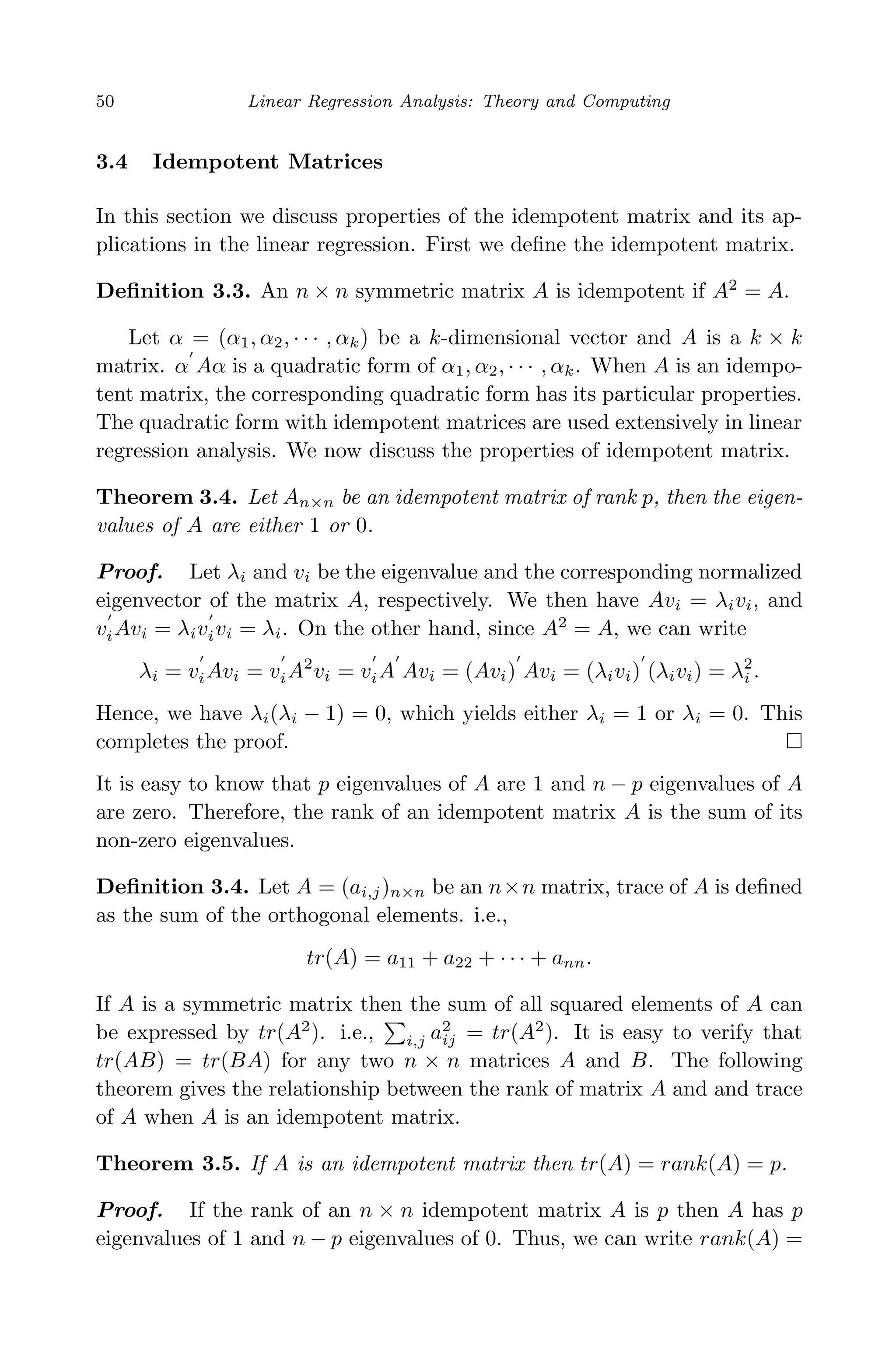
Multiple Linear Regression 85
Since the eigenvalues of (X X)−1
are
1
λ1
,
1
λ2
, · · · ,
1
λk
we have
E(b b) = β β + σ2
k
i=1
1
λi
,
or it can be written as
E
k
i=1
b2
i =
k
i=1
β2
i + σ2
k
i=1
1
λi
. (3.39)
Now it is easy to see that if one of λ is very small, say, λi = 0.0001, then
roughly,
k
i=1 b2
i may over-estimate
k
i=1 β2
i by 1000σ2
times. The above
discussions indicate that if some columns in X are highly correlated with
other columns in X then the covariance matrix (XX )−1
σ2
will have one
or more large eigenvalues so that the mean Euclidean distance of E[(b −
β) (b − β)] will be inflated. Consequently, this makes the estimation of
the regression parameter β less reliable. Thus, the collinearity in column
vectors of X will have negative impact on the least squares estimates of
regression parameters and this need to be examined carefully when doing
regression modeling.
How to deal with the collinearity in the regression modeling? One easy
way to combat collinearity in multiple regression is to centralize the data.
Centralizing the data is to subtract mean of the predictor observations from
each observation. If we are not able to produce reliable parameter estimates
from the original data set due to collinearity and it is very difficult to judge
whether one or more independent variables can be deleted, one possible
and quick remedy to combat collinearity in X is to fit the centralized data
to the same regression model. This would possibly reduce the degree of
collinearity and produce better estimates of regression parameters.
3.17.2 Variance Inflation
Collinearity can be checked by simply computing the correlation matrix of
the original data X. As we have discussed, the variance inflation of the
least squares estimator in multiple linear regression is caused by collinearity
of the column vectors in X. When collinearity exists, the eigenvalues of
the covariance matrix (X X)−1
σ2
become extremely large, which causes
severe fluctuation in the estimates of regression parameters and makes these](https://image.slidesharecdn.com/xinyanxiaogangsulinearregressionanalysisbookfi-140714092751-phpapp02/75/Xin-yan-xiao_gang_su-_linear_regression_analysis-book_fi-org-106-2048.jpg)

![April 29, 2009 11:50 World Scientific Book - 9in x 6in Regression˙master
106 Linear Regression Analysis: Theory and Computing
Proof. For the regression model without using the ith observation the
residual is
ei,−i = yi − xib−i = yi − xi(X−iX−i)−1
X−iy−i
= yi − xi (X X)−1
+
(X X)−1
xixi(X X)−1
1 − hii
X−iy−i
=
(1 − hii)yi − (1 − hii)xi(X X)−1
X−iy−i − hiixi(X X)−1
X−iy−i
1 − hii
=
(1 − hii)yi − xi(X X)−1
X−iy−i
1 − hii
Note that X−iy−i + xiyi = X y we have
ei,−i =
(1 − hii)yi − xi(X X)−1
(X y − xiyi)
1 − hii
=
(1 − hii)yi − xi(X X)−1
X y + xi(X X)−1
xiyi
1 − hii
=
(1 − hii)yi − ˆyi + hiiyi
1 − hii
=
yi − ˆyi
1 − hii
=
ei
1 − hii
For variance of PRESS residual Var(ei,−i) we have
Var(ei,−i) = Var(ei)
1
(1 − hii)2
= [σ2
(1 − hii)]
1
(1 − hii)2
=
σ2
1 − hii
The ith standardized PRESS residual is
ei,−i
σi,−i
=
ei
σ
√
1 − hii
. (3.76)
3.20.5 Identify Outlier Using PRESS Residual
The standardized PRESS residual can be used to detect outliers since it is
related to the ith observation and is scale free. If the ith PRESS residual
is large enough then the ith observation may be considered as a potential
outlier. In addition to looking at the magnitude of the ith PRESS residual,
according to the relationship between the PRESS residual ei,−i and the
regular residual ei, the ith observation may be a potential outlier if the
leverage hii is close to 1.](https://image.slidesharecdn.com/xinyanxiaogangsulinearregressionanalysisbookfi-140714092751-phpapp02/75/Xin-yan-xiao_gang_su-_linear_regression_analysis-book_fi-org-127-2048.jpg)


![April 29, 2009 11:50 World Scientific Book - 9in x 6in Regression˙master
Detection of Outliers and Influential Observations in Multiple Linear Regression 131
would be the model with R2
value close to 1. If the data fit well the
regression model then it should be expected that yi is close enough to
ˆyi. Hence, SSRes should be fairly close to zero. Therefore, R2
should
be close to 1.
2. Estimate of error variance s2
. Among a set of possible regression models
a preferred regression model should be one that has a smaller value of
s2
since this corresponds to the situation where the fitted values are
closer to the response observations as a whole.
3. Adjusted ¯R2
. Replace SSRes and SST otal by their means:
¯R2
= 1 −
SSRes/n − p
SST otal/n − 1
= 1 −
s2
(n − 1)
SST otal
Note that SST otal is the same for all models and the ranks of R2
for all
models are the same as the ranks of s2
for all models. We would like
to choose a regression model with adjusted ¯R2
close to 1.
4.1.2 Bias in Error Estimate from Under-specified Model
We now discuss the situation where the selected model is under-specified.
i.e.,
y = X1β1 + ε. (4.1)
Here, the under-specified model is a model with inadequate regressors. In
other words, if more regressors are added into the model, the linear com-
bination of the regressors can better predict the response variable. Some-
times, the under-specified model is also called as reduced model. Assuming
that the full model is
y = X1β1 + X2β2 + ε, (4.2)
and the number of parameters in the reduced model is p, let s2
p be the error
estimate based on the under-specified regression model. The fitted value
from the under-specified regression model is
ˆy = X1(X1X1)−1
X1y
and error estimate from the under-specified regression model is
s2
p = y (I − X1(X1X1)−1
X1)y.
We then compute the expectation of the error estimate s2
p.
E(s2
p) = σ2
+
β2[X2X2 − X2X1(X1X1)−1
X2X1]β2
n − p
. (4.3)](https://image.slidesharecdn.com/xinyanxiaogangsulinearregressionanalysisbookfi-140714092751-phpapp02/75/Xin-yan-xiao_gang_su-_linear_regression_analysis-book_fi-org-152-2048.jpg)


![April 29, 2009 11:50 World Scientific Book - 9in x 6in Regression˙master
Model Diagnostics 199
is defined as
LR = 2[log l(x, ˆθ) − log l(x, ˜θ)], (6.3)
where ˆθ is the likelihood estimate without restrictions, ˜θ is the likelihood
estimate with restrictions, and g is the number of the restrictions imposed.
The asymptotic distribution of the LR test is the χ2
with g degrees of
freedom. The Wald test is defined as
W = (ˆθ − θ0) I(ˆθ)(ˆθ − θ0), (6.4)
where I(θ) = Eθ
∂2
log l(x, θ)
∂θ2
, the information matrix.
The basic idea of the Lagrange multiplier test focuses on the characteristic
of the log-likelihood function when the restrictions are imposed on the null
hypothesis. Suppose that the null hypothesis is H0 : β = β0, we consider
a maximization problem of log-likelihood function when the restriction of
the null hypothesis which we believe to be true is imposed. That is, we
try to solve for maximization problem under the constrain β = β0. This
restricted maximization problem can be solved via the Lagrange multiplier
method. i.e., we can solve for the unconstrained maximization problem:
max
β
L(β) + λ(β − β0) .
Differentiating with respect to β and λ and setting the results equal to
zero yield the restricted maximum likelihood estimation, β∗
= β0, and the
estimate of the Lagrange multiplier, λ∗
= S(β∗
) = S(β0), where S(·) is
the slope of the log-likelihood function, S(β) =
dL(β)
dβ
, evaluated at the
restricted value β0. The greater the agreement between the data and the
null hypothesis, i.e., ˆβ ≈ β0, the closer the slope will be to zero. Hence,
the Lagrange multiplier can be used to measure the distance between ˆβ
and β0. The standard form for the LM test is defined as
LM = [S(θ0)]2
I(θ0)−1
∼ χ2
1 (6.5)
The generalization to the multivariate version is a straightforward extension
of (6.5) and can be written as
LM = S(˜θ) I(˜θ)−1
S(˜θ) ∼ χ2
g, (6.6)
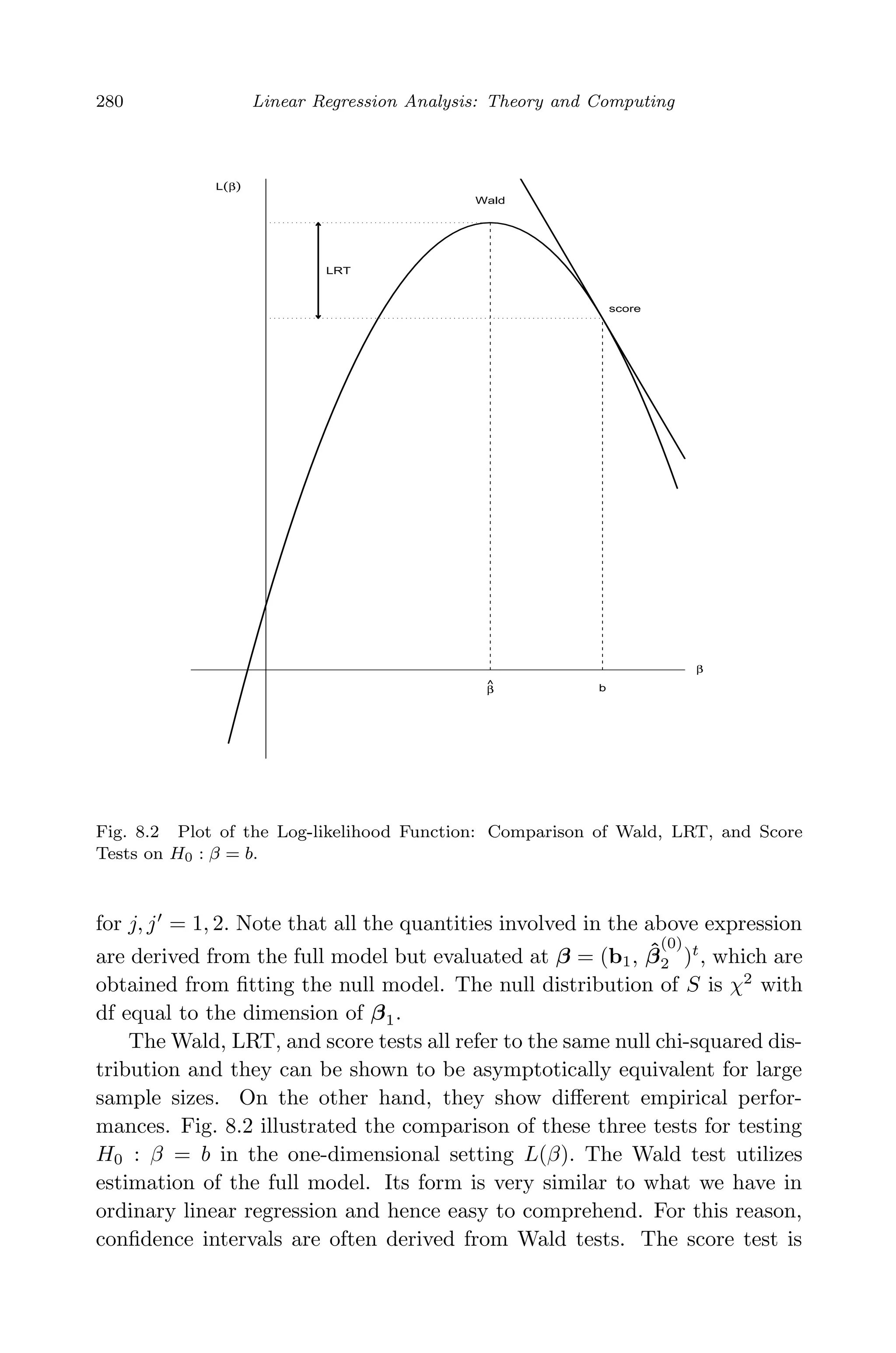
where g is the number of linear restrictions imposed.](https://image.slidesharecdn.com/xinyanxiaogangsulinearregressionanalysisbookfi-140714092751-phpapp02/75/Xin-yan-xiao_gang_su-_linear_regression_analysis-book_fi-org-220-2048.jpg)
![April 29, 2009 11:50 World Scientific Book - 9in x 6in Regression˙master
200 Linear Regression Analysis: Theory and Computing
Example We now give an example to compute the LR, Wald, and LM
tests for the elementary problem of the null hypothesis H0 : µ = µ0 against
Ha : µ = µ0 from a sample size n drawn from a normal distribution with
variance of unity. i.e., X ∼ N(µ, 1) and the log-likelihood function is
L(µ) = −
n
2
log(2π) −
1
2
n
i=1
(Xi − µ)2
,
which is a quadratic form in µ. The first derivative of the log-likelihood is
dL(µ)
dµ
=
n
i=1
(Xi − µ) = n( ¯X − µ),
and the first derivative of the log-likelihood is a quadratic form in µ. The
second derivative of the log-likelihood is a constant:
d2
L(µ)
dµ2
= −n.
The maximum likelihood estimate of µ is ˆµ = ¯X and LR test is given by
LR = 2[L(ˆµ) − L(µ0)]
=
n
i=1
(Xi − µ0)2
−
n
i=1
(Xi − ¯X)2
= n( ¯X − µ0)2
. (6.7)
The Wald test is given by
W = (µ − µ0)2
I(θ0) = n( ¯X − µ0)2
. (6.8)
Since
dL(µ0)
dµ
= n( ¯X − µ0), the LM test is given by
W = S(µ0)2
C(θ0)−1
= n( ¯X − µ0)2
. (6.9)
Note that ¯X ∼ N(µ0, n−1
), each statistic is the square of a standard normal
variable and hence is distributed as χ2
with one degree of freedom. Thus,
in this particular example the test statistics are χ2
for all sample sizes and
therefore are also asymptotically χ2
1.](https://image.slidesharecdn.com/xinyanxiaogangsulinearregressionanalysisbookfi-140714092751-phpapp02/75/Xin-yan-xiao_gang_su-_linear_regression_analysis-book_fi-org-221-2048.jpg)


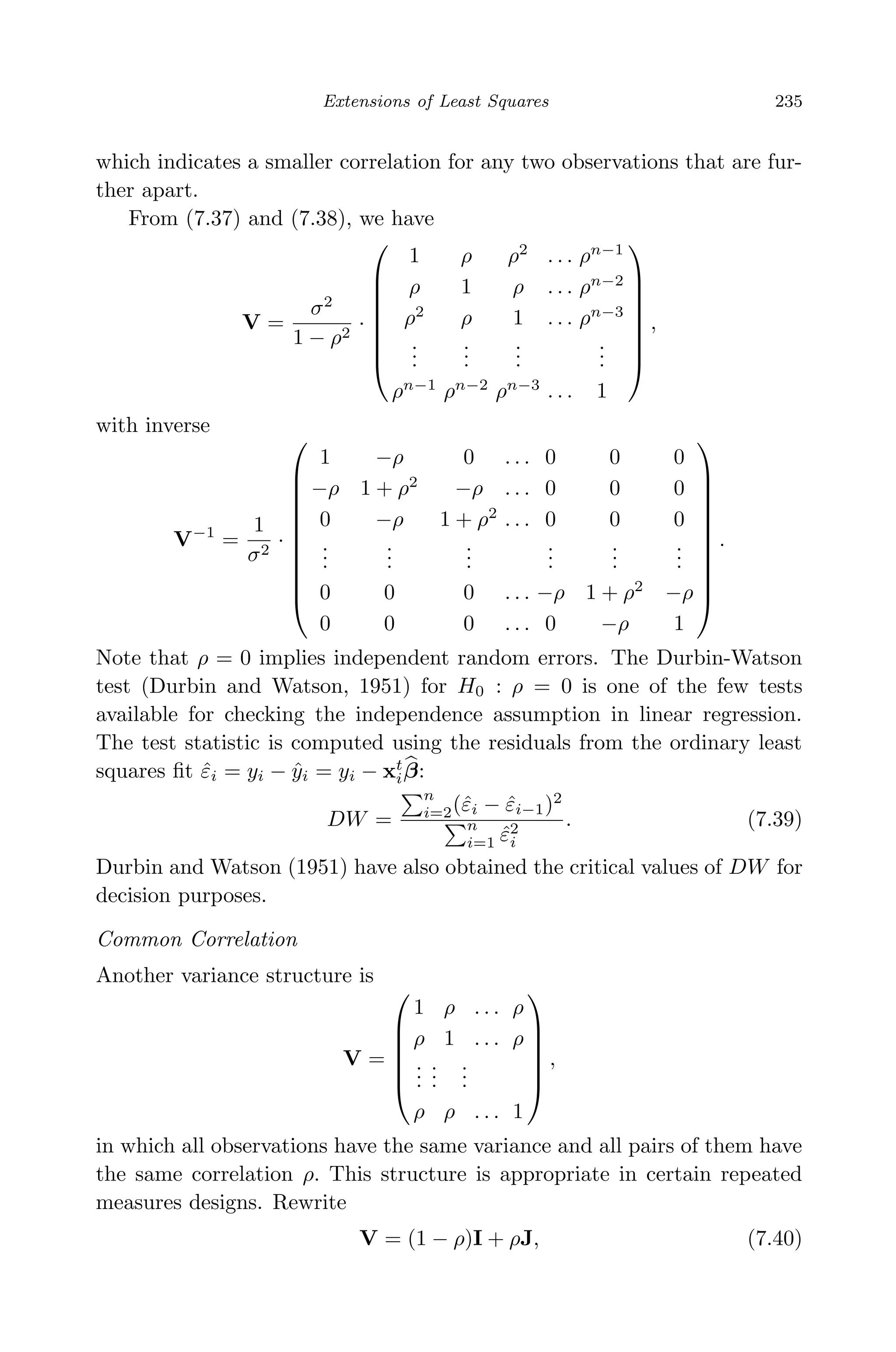
![April 29, 2009 11:50 World Scientific Book - 9in x 6in Regression˙master
234 Linear Regression Analysis: Theory and Computing
of β. Based on the residuals, the weights are re-estimated and the WLS
estimation is updated. The process is iterated until the WLS fit gets stable.
AR(1) Variance Structure
Variance structures from time series models can be employed to model
data collected over time in longitudinal studies. Consider a multiple linear
regression model with random errors that follow a first-order autoregressive
process:
yi = xt
iβ + εi with εi = ρεi−1 + νi, (7.36)
where νi ∼ N(0, σ2
) independently and −1 < ρ < 1.
To find out the matrix V, we first rewrite εi
εi = ρ · εi−1 + νi
= ρ · (ρεi−2 + νi−1) + νi
= νt + ρνi−1 + ρ2
νi−2 + ρ3
νi−3 + · · ·
=
∞
s=0
ρs
νi−s.
It follows that E(εi) =
∞
s=0 ρs
E(νi−s) = 0 and
Var(εi) =
∞
s=0
ρ2s
Var(νi−s) = σ2
∞
s=0
ρ2s
=
σ2
1 − ρ2
. (7.37)
Furthermore, the general formula for the covariance between two observa-
tions can be derived. Consider
Cov(εi, εi−1) = E(εiεi−1) = E {(ρ εi−1 + νi) · εi−1}
= E ρ ε2
i−1 + νiεi−1 = ρ · E(ε2
i−1)
= ρ · Var(εi−1) = ρ ·
σ2
1 − ρ2
Also, using εi = ρ · εi−1 + νi = ρ · (ρεi−2 + νi−1) + νi, it can be found that
Cov(εi, εi−2) = E(εiεi−2) = E [{ρ · (ρεi−2 + νi−1) + νi} · εi−2]
= ρ2
·
σ2
1 − ρ2
.
In general, the covariance between error terms that are s steps apart is
Cov(εi, εi−s) = ρs σ2
1 − ρ2
. (7.38)
Thus, the correlation coefficient is
cov(εi, εi−s) = ρs
,](https://image.slidesharecdn.com/xinyanxiaogangsulinearregressionanalysisbookfi-140714092751-phpapp02/75/Xin-yan-xiao_gang_su-_linear_regression_analysis-book_fi-org-255-2048.jpg)
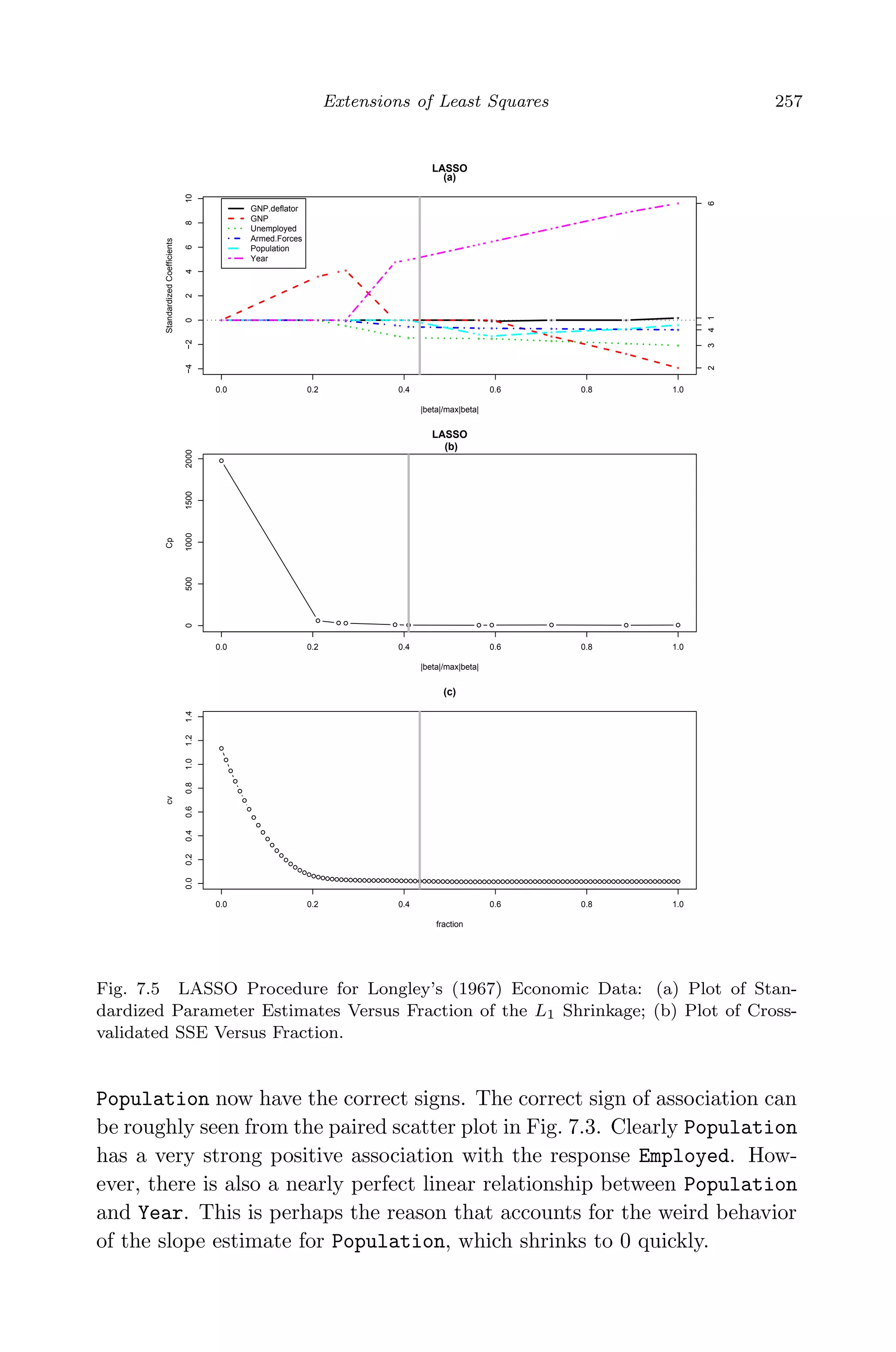
![May 7, 2009 10:22 World Scientific Book - 9in x 6in Regression˙master
258 Linear Regression Analysis: Theory and Computing
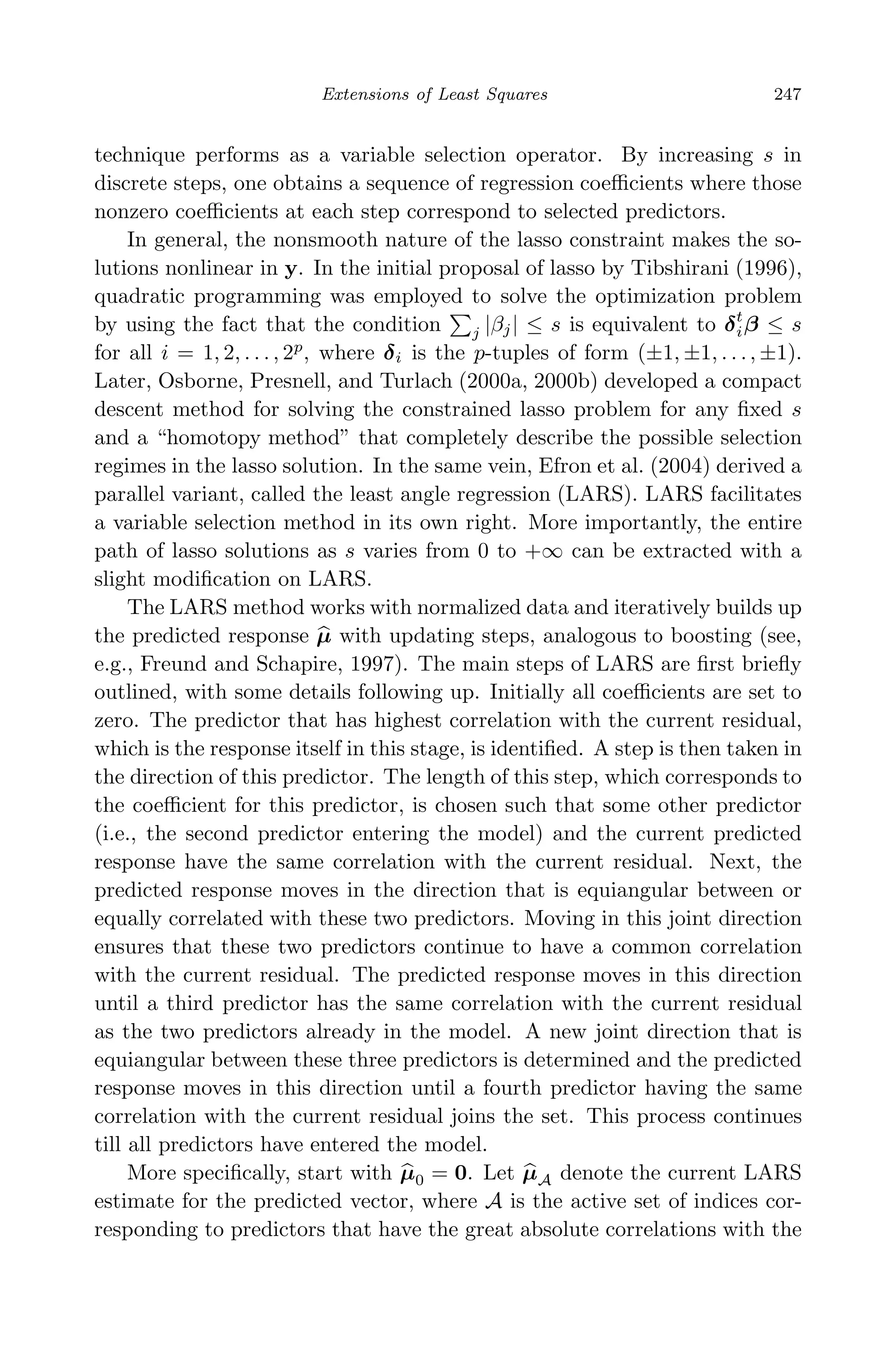
Finally, we obtained the LASSO estimation via the LARS implemen-
tation. Figure 7.5(a) depicts the LASSO trace, which is the plot of the
standardized coefficients versus s, expressed in the form of a fraction
j |ˆβlasso
j |/ j |ˆβLS
j |. Compared to the ridge trace, we see some similar per-
formance of the slope estimates, e.g., the sign change of GNP, the suppression
of GNP.deflator, the relative stability of Armed.Forces and Unemployed,
the prominent positive effect of Year. The most striking difference, how-
ever, is that there are always some zero coefficients for a given value of
s ∈ [0, 1], which renders lasso an automatic variable selector.
Two methods are suggested by Efron et al. (2004) to determine an
optimal s. The first is to apply a Cp estimate for prediction error. Efron
et al. (2004) found that the effective number of degrees of freedom involved
in lasso can be well approximated simply by k0, the number of predictors
with nonzero coefficients. The Cp criterion is then given by
Cp(s) =
SSE(s)
ˆσ2
− n + 2k0,
where, SSE(s) is the resulting sum of squared errors from LASSO fit for a
given value of s and ˆσ2
is the unbiased estimate of σ2
from OLS fitting of the
full model. The second method is through v-fold cross validation. In this
approach, the data set is randomly divided into v equally-sized subsets. For
observations in each subset, their predicted values ˆyCV
are computed based
on the model fit using the other v − 1 subsets. Then the cross-validated
sum of squared errors is i(yi − ˆyCV
i )2
. Figure 7.5 (b) and (c) plot the
Cp values and 10-fold cross-validated sum of squared errors, both versus s.
The minimum Cp yields an optimal fraction of 0.41, which is very close to
the choice, 0.43, selected by minimum cross-validated SSE.
With a fixed s, the standard errors of LASSO estimates can be com-
puted either via bootstrap (Efron and Tibshirani, 1993) or by analytical
approximation. In the bootstrap or resampling approach, one generates B
replicates, called bootstrap samples, from the original data set by sampling
with replacement. For the b-th bootstrap sample, the LASSO estimate β
lasso
b
is computed. Then the standard errors of lasso estimates are computed as
the sample standard deviation of β
lasso
b ’s. Tibshirani (1996) derived an ap-
proximate close form for the standard errors by rewriting the lasso penalty
|βj| as β2
j /|βj|. The lasso solution can then be approximated by a
ridge regression of form
β
lasso
≈ (Xt
X + kW−
)−1
Xt
y, (7.78)
where W is a diagonal matrix with diagonal elements | ˆβj
lasso
|; W−
denotes
a generalized inverse of W; and k is chosen so that | ˆβj
lasso
| = s. The](https://image.slidesharecdn.com/xinyanxiaogangsulinearregressionanalysisbookfi-140714092751-phpapp02/75/Xin-yan-xiao_gang_su-_linear_regression_analysis-book_fi-org-279-2048.jpg)

![May 7, 2009 10:22 World Scientific Book - 9in x 6in Regression˙master
Generalized Linear Models 271
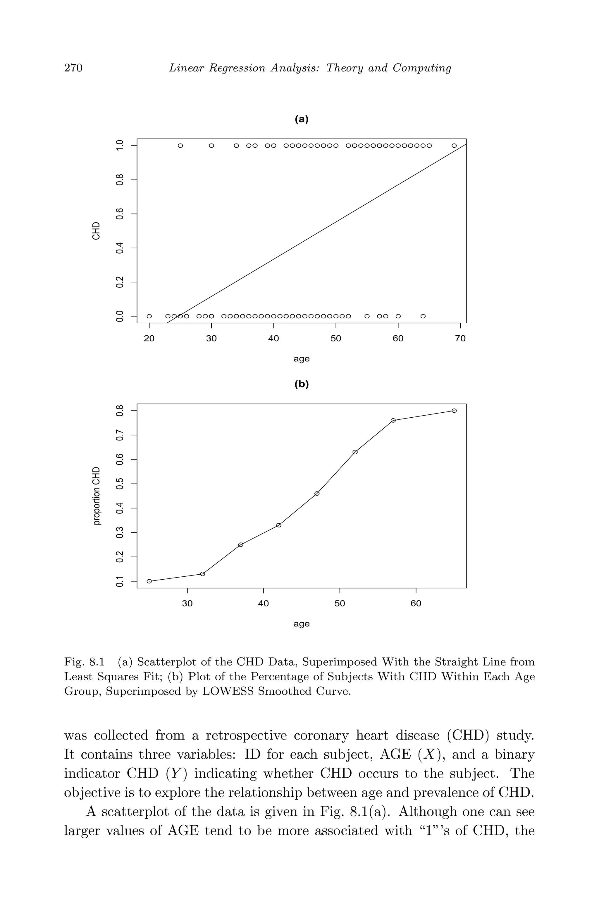
plot is not very informative due to discreteness of the response Y .
Recall that linear regression relates the conditional mean of the re-
sponse, E(Y |X), to a linear combination of predictors. Can we do the
same with binary data? Let the binary response yi = 1 if CHD is found in
the ith individual and 0 otherwise for i = 1, . . . , n. Denote πi = Pr(yi = 1).
Thus, the conditional distribution of yi given xi is a Bernoulli trial with
parameter πi. It can be found that E(yi) = πi. Hence, the linear model
would be
E(yi) = πi = β0 + β1xi. (8.1)
Figure 8.1(a) plots the straight line fitted by least squares. Clearly, it is
not a good fit. There is another inherent problem with Model (8.1). The
left-hand side πi ranges from 0 to 1, which does not mathematically match
well with the range (−∞, ∞) of the linear equation on the right-hand side.
A transformation on πi, g(·), which maps [0, 1] onto (−∞, ∞), would help.
This transformation function is referred to the link function.
In order to explore the functional form between πi and xi, we must
have available estimates of the proportions πi. One approach is group the
data by categorizing AGE into several intervals and record the relatively
frequency of CHD within each interval. Table 8.1 shows the worksheet for
this calculation.
Table 8.1 Frequency Table of AGE Group by CHD.
CHD
Age Group n Absent Present Proportion
20-29 10 9 1 0.10
30-34 15 23 2 0.13
35-39 12 9 3 0.25
40-44 15 10 5 0.33
45-49 13 7 6 0.46
50-54 8 3 5 0.63
55-59 17 4 13 0.76
60-69 10 2 8 0.80
Total 100 57 43 0.43
Figure 8.1(b) plots the proportions of subjects with CHD in each age
interval versus the middle value of the interval. It can be seen that the
conditional mean of yi or proportion gradually approaches zero and one to
each end. The plot shows an ‘S’-shaped or sigmoid nonlinear relationship,
in which the change in π(x) with per unit increase in x grows quickly at first,
but gradually slows down and then eventually levels off. Such a pattern is](https://image.slidesharecdn.com/xinyanxiaogangsulinearregressionanalysisbookfi-140714092751-phpapp02/75/Xin-yan-xiao_gang_su-_linear_regression_analysis-book_fi-org-292-2048.jpg)
![April 29, 2009 11:50 World Scientific Book - 9in x 6in Regression˙master
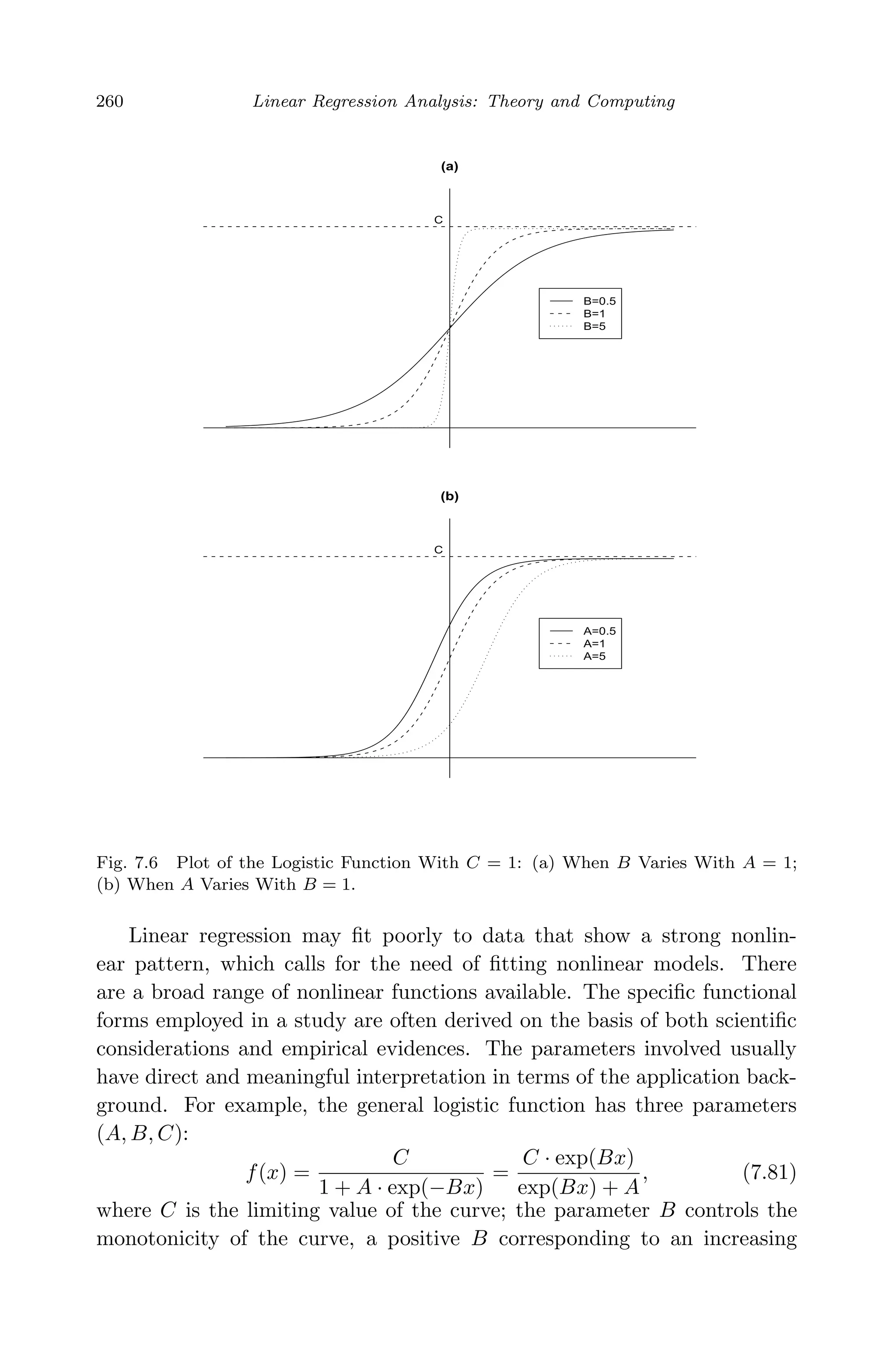
272 Linear Regression Analysis: Theory and Computing
rather representative and can be generally seen in many other applications.
It is often expected to see that a fixed change in x has less impact when
π(x) is near 0 or 1 than when π(x) is near 0.5. Suppose, for example, that
π(x) denotes the probability to pass away for a person of age x. An increase
of five years in age would have less effect on π(x) when x = 70, in which
case π(x) is perhaps close to 1, than when x = 40.
In sum, a suitable link function g(πi) is desired to satisfy two conditions:
it maps [0, 1] onto the whole real line and has the sigmoid shape. A natural
choice for g(·) would be a cumulative distribution function of a random
variable. In particular, the logistic distribution, whose CDF is the simplified
logistic function g(x) = exp(x)/{1 + exp(x)} in (7.81), yields the most
popular link. Under the logistic link, the relationship between the CHD
prevalence rate and AGE can be formulated by the following simple model
logit(πi) = log
πi
1 − πi
= β0 + β1xi.
When several predictors {X1, . . . , Xp} are involved, the multiple logistic
regression can be generally expressed as
log
πi
1 − πi
= xiβ.
We shall explore more on logistic regression in Section 8.5.
8.2 Components of GLM
The logistic regression model is one of the generalized linear models (GLM).
Many models in the class had been well studied by the time when Nelder
and Wedderburn (1972) introduced the unified GLM family. The specifica-
tion of a GLM generally consists of three components: a random component
specifies the probability distribution of the response; a systematic compo-
nent forms the linear combination of predictors; and a link function relates
the mean response to the systematic component.
8.2.1 Exponential Family
The random component assumes a probability distribution for the response
yi. This distribution is taken from the natural exponential distribution
family of form
f(yi; θi, φ) = exp
yiθi − b(θi)
a(φ)
+ c(yi; φ) , (8.2)](https://image.slidesharecdn.com/xinyanxiaogangsulinearregressionanalysisbookfi-140714092751-phpapp02/75/Xin-yan-xiao_gang_su-_linear_regression_analysis-book_fi-org-293-2048.jpg)
![April 29, 2009 11:50 World Scientific Book - 9in x 6in Regression˙master
Generalized Linear Models 285
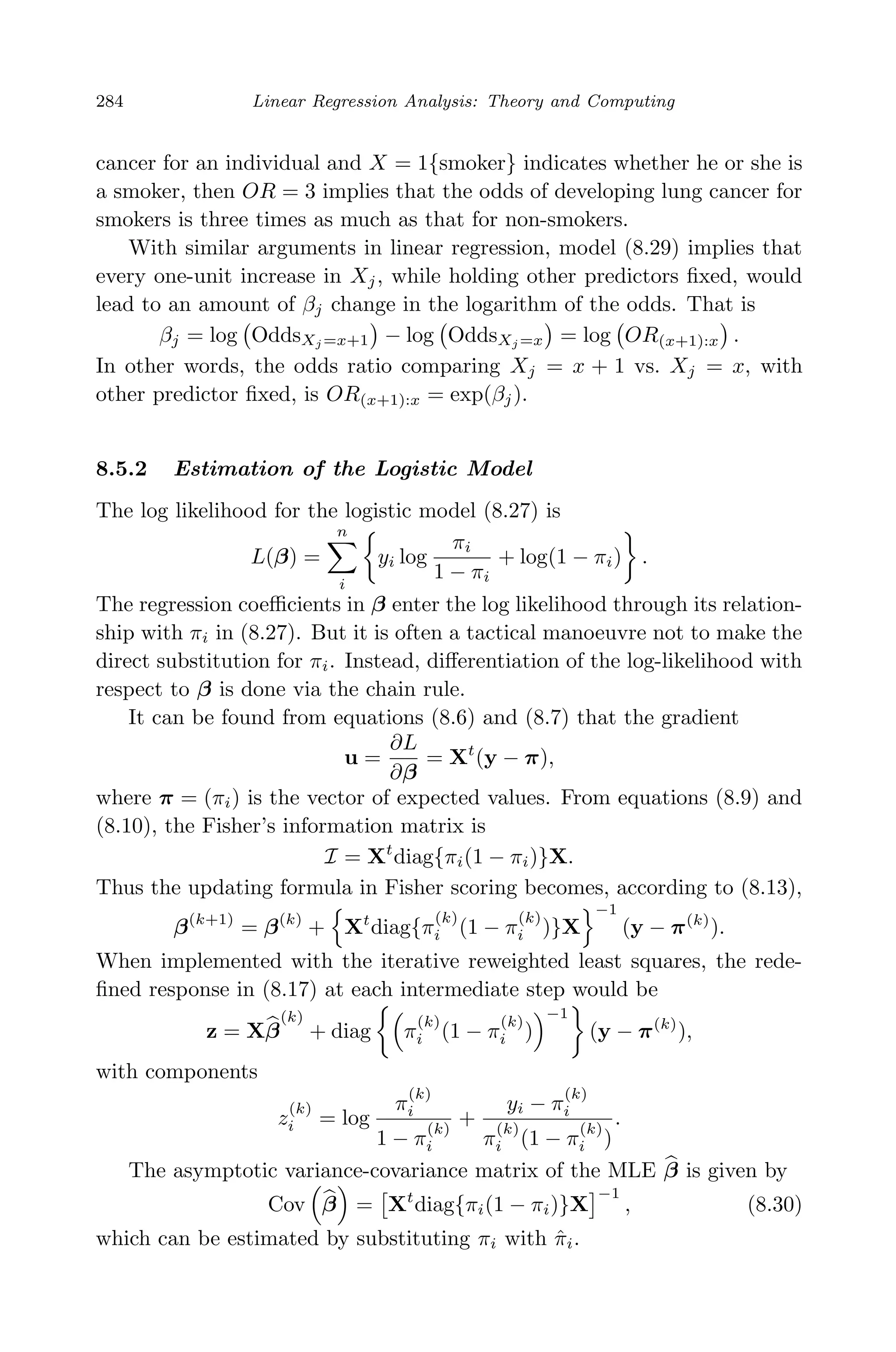
8.5.3 Example
To illustrate, we consider the kyphosis data (Chambers and Hastie, 1992)
from a study of children who have had corrective spinal surgery. The data
set contains 81 observations and four variables. A brief variable description
is given below. The binary response, kyphosis, indicates whether kyphosis,
a type of deformation was found on the child after the operation.
Table 8.2 Variable Description for the Kyphosis Data: Logistic
Regression Example.
kyphosis indicating if kyphosis is absent or present;
age age of the child (in months);
number number of vertebrae involved;
start number of the first (topmost) vertebra operated on.
Logistic regression models can be fit using PROC LOGISTIC, PROC
GLM, PROC CATMOD, and PROC GENMOD in SAS. In R, the function
glm in the base library can be used. Another R implementation is also
available in the package Design. In particular, function lrm provides pe-
nalized maximum likelihood estimation, i.e., the ridge estimator, for logistic
regression.
Table 8.1 presents some selected fitting results from PROC LOGISTIC
for model
log
P(kyphosis = 1)
P(kyphosis = 0)
= β0 + β1 · age + β2 · number + β3 · start.
Panel (a) gives the table of parameter estimates. The fitted logistic model
is
logit{P(kyphosis = 1)} = −2.0369 + 0.0109 × age + 0.4106 × number
−0.2065 × start.
Accordingly, prediction of P(kyphosis = 1) can be obtained using (8.28).
Panel (b) provides the estimates for the odds ratios (OR), exp(ˆβj), and
the associated 95% confidence intervals. The confidence interval for OR
is constructed by taking the exponential of the lower and upper bounds
of the confidence interval for β. Based on the results, we can conclude
with 95% confidence that the odds of having kyphosis would be within
[0.712, 0.929] times if the number of the first (topmost) vertebra operated
on, start, increases by one, for children with same fixed age and number
values. Since 1 is not included in this confidence interval, the effect of](https://image.slidesharecdn.com/xinyanxiaogangsulinearregressionanalysisbookfi-140714092751-phpapp02/75/Xin-yan-xiao_gang_su-_linear_regression_analysis-book_fi-org-306-2048.jpg)
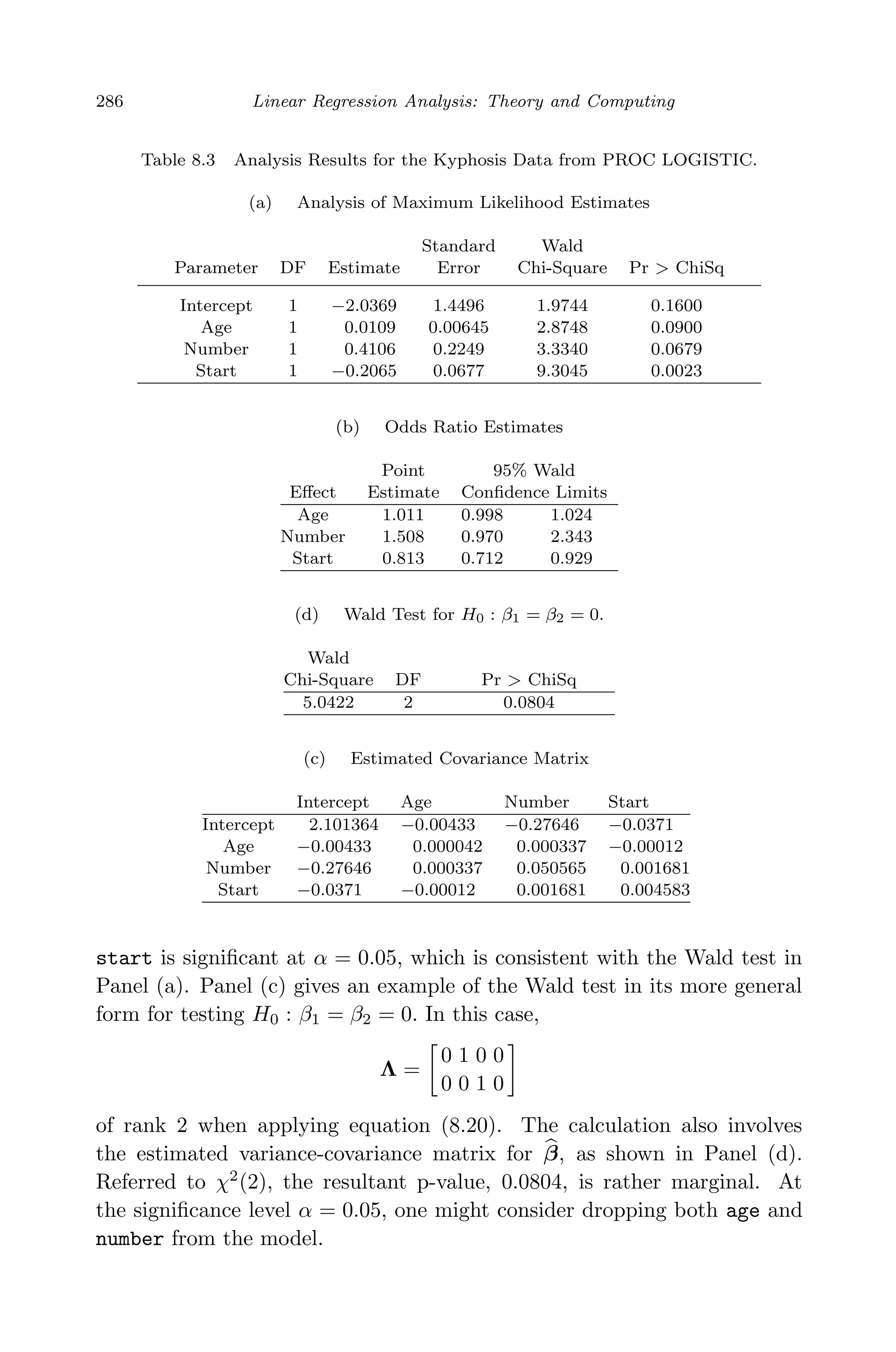


![April 29, 2009 11:50 World Scientific Book - 9in x 6in Regression˙master
312 Linear Regression Analysis: Theory and Computing
provides the best predictions, then it should be effectively discredited and
hence not be considered. Under this principal, they exclude models in set
A1 = Mk :
maxl{pr(Ml|D)}
pr(Mk|D)
> C , (9.45)
for some user-defined threshold C. Moreover, they suggested to exclude
complex models which receive less support from the data than their simpler
counterparts, a principle appealing to Occam’s razor. Namely, models in
set
A2 = Mk : ∃ Ml /∈ A1, Ml ⊂ Mk and
pr(Ml|D)
pr(Mk|D)
> 1 (9.46)
could also be excluded from averaging. The notation Ml ⊂ Mk means
that Ml is nested into or a sub-model of Mk. This strategy greatly reduces
the number of models and all the probabilities in (9.35) – (9.37) are then
implicitly conditional on the reduced set. The second approach, called
Markov chain Monte Carlo model composition (MC3
) due to Madigan and
York (1995), approximates the posterior distribution in (9.35) numerically
with a Markov chain Monte Carlo procedure.
One additional issue in implementation of BMA is how to assign the
prior model probabilities. When little prior information about the relative
plausibility of the models consider, a noninformative prior that treats all
models equally likely is advised. When prior information about the impor-
tance of a variable is available for model structures that have a coefficient
associated with each predictor (e.g., linear regression), a prior probability
on model Mk can be specified as
pr(Mk) =
p
j=1
π
δkj
j (1 − πj)1−δkj
, (9.47)
where πj ∈ [0, 1] is the prior probability that βj = 0 in a regression model,
and δki is an indicator of whether or not Xj is included in model Mk. See
Raftery, Madigan, and Hoeting (1997) and Hoeting et al. (1999) for more
details and other issues in BMA implementation. BMA is available in the
R package BMA.
Example We revisit the quasar example with an analysis of BMA in
Chapter 5. The data set, given in Table 5.1, involves 5 predictors. Thus
there are a total of 25
= 32 linear models under consideration. With a
threshold C = 40 in (9.46), 13 models are selected according to Occam’s
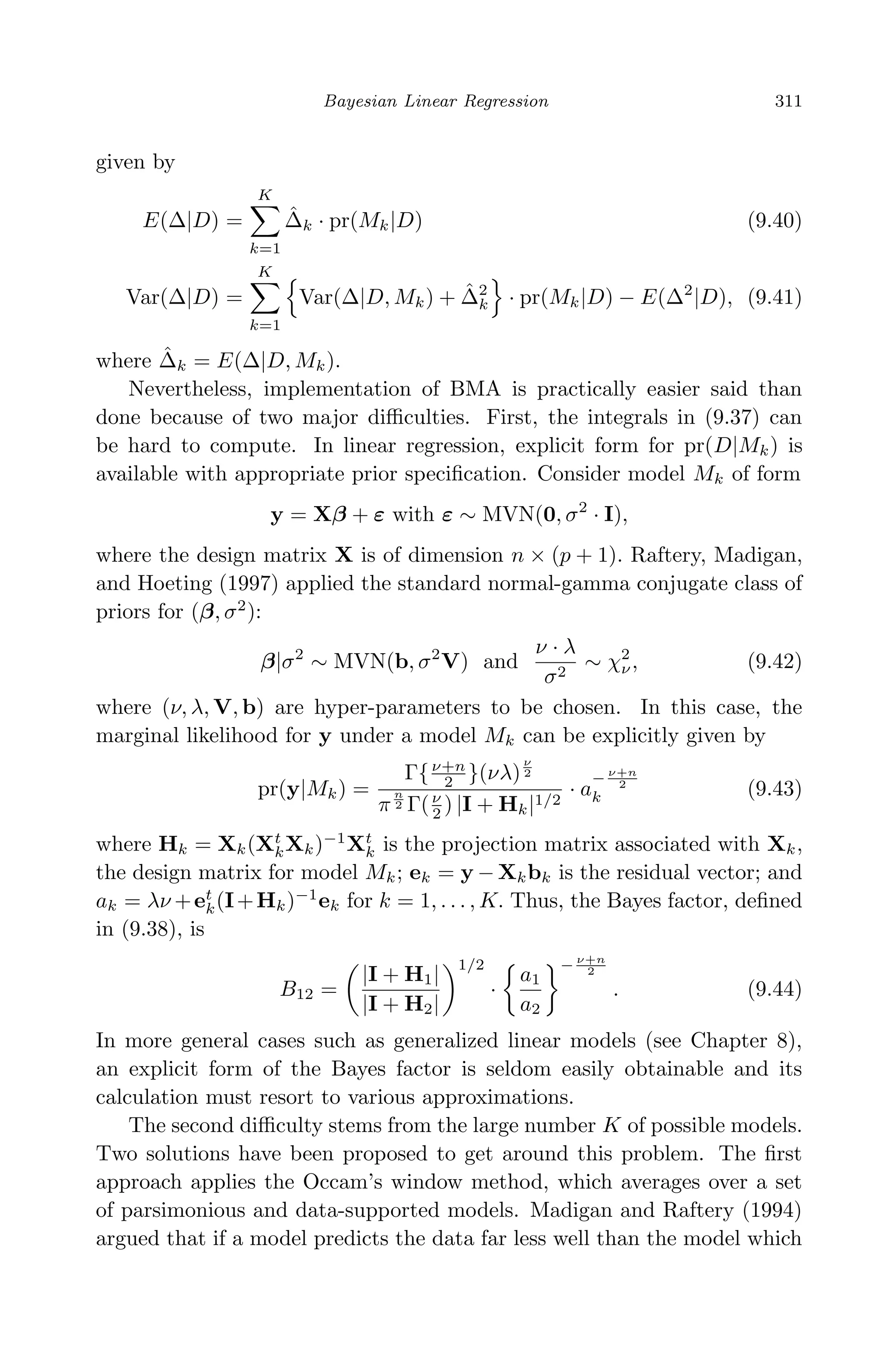
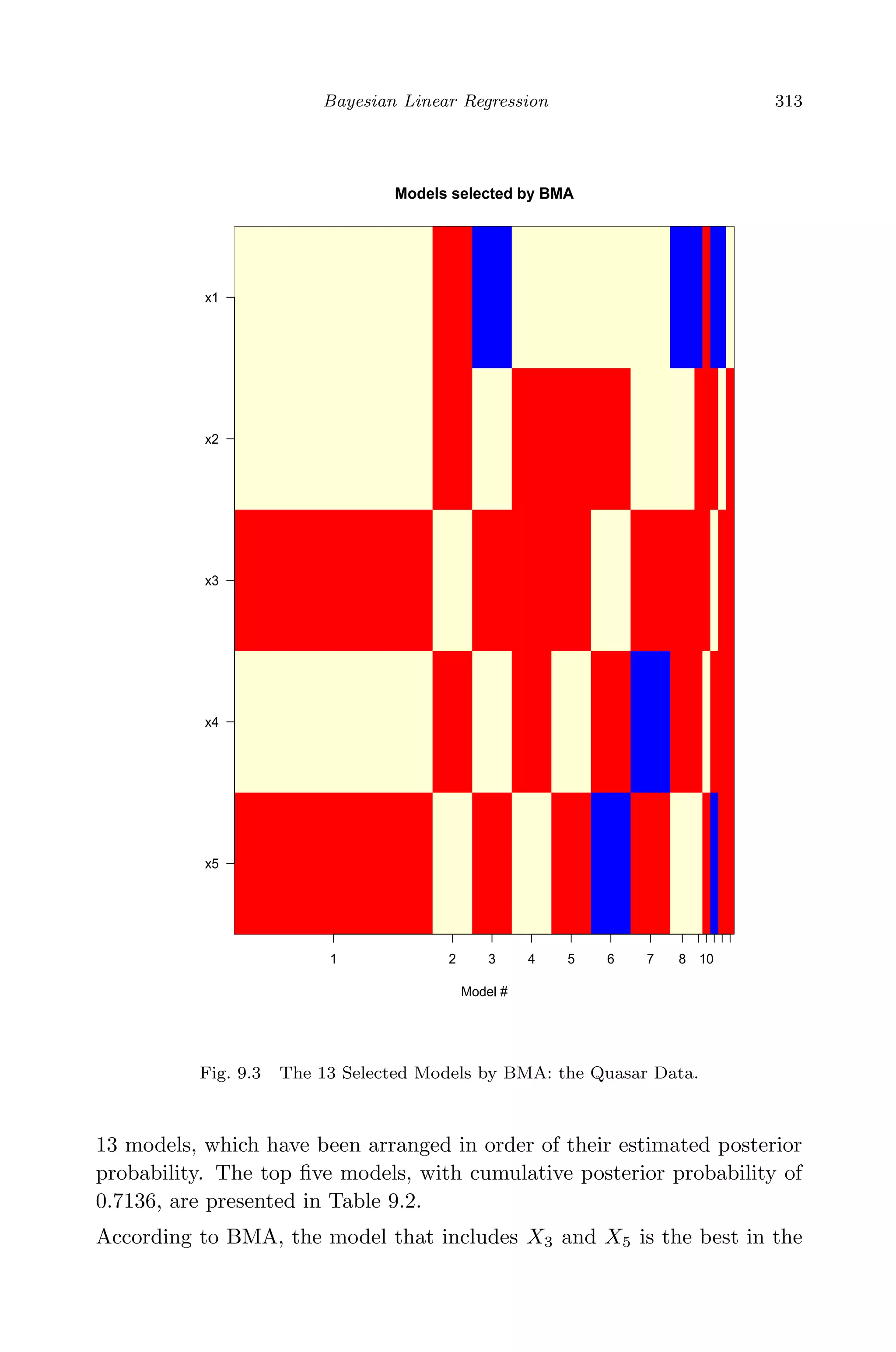
window. Figure 9.3 shows the variable selection information for all the](https://image.slidesharecdn.com/xinyanxiaogangsulinearregressionanalysisbookfi-140714092751-phpapp02/75/Xin-yan-xiao_gang_su-_linear_regression_analysis-book_fi-org-333-2048.jpg)


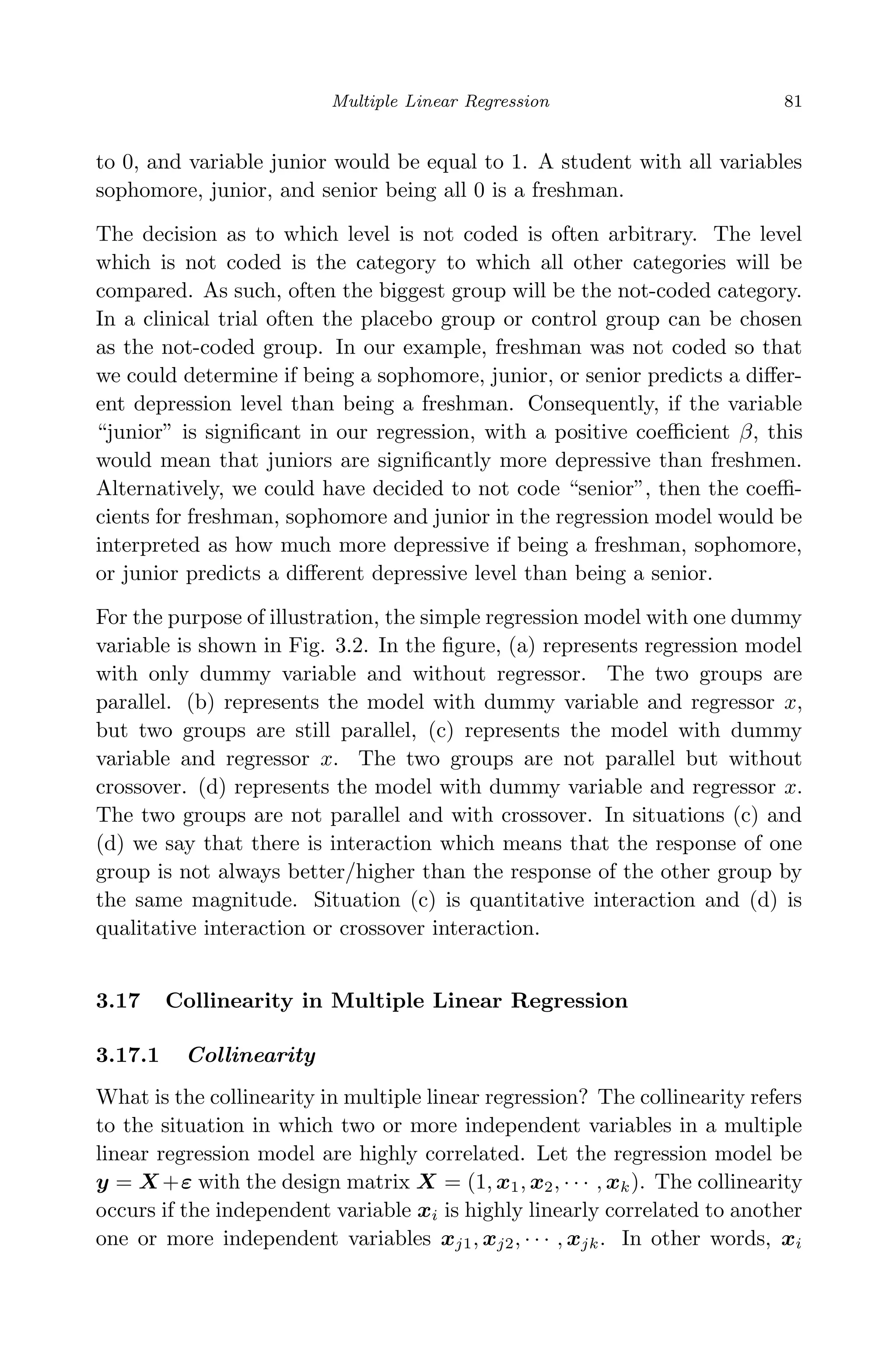
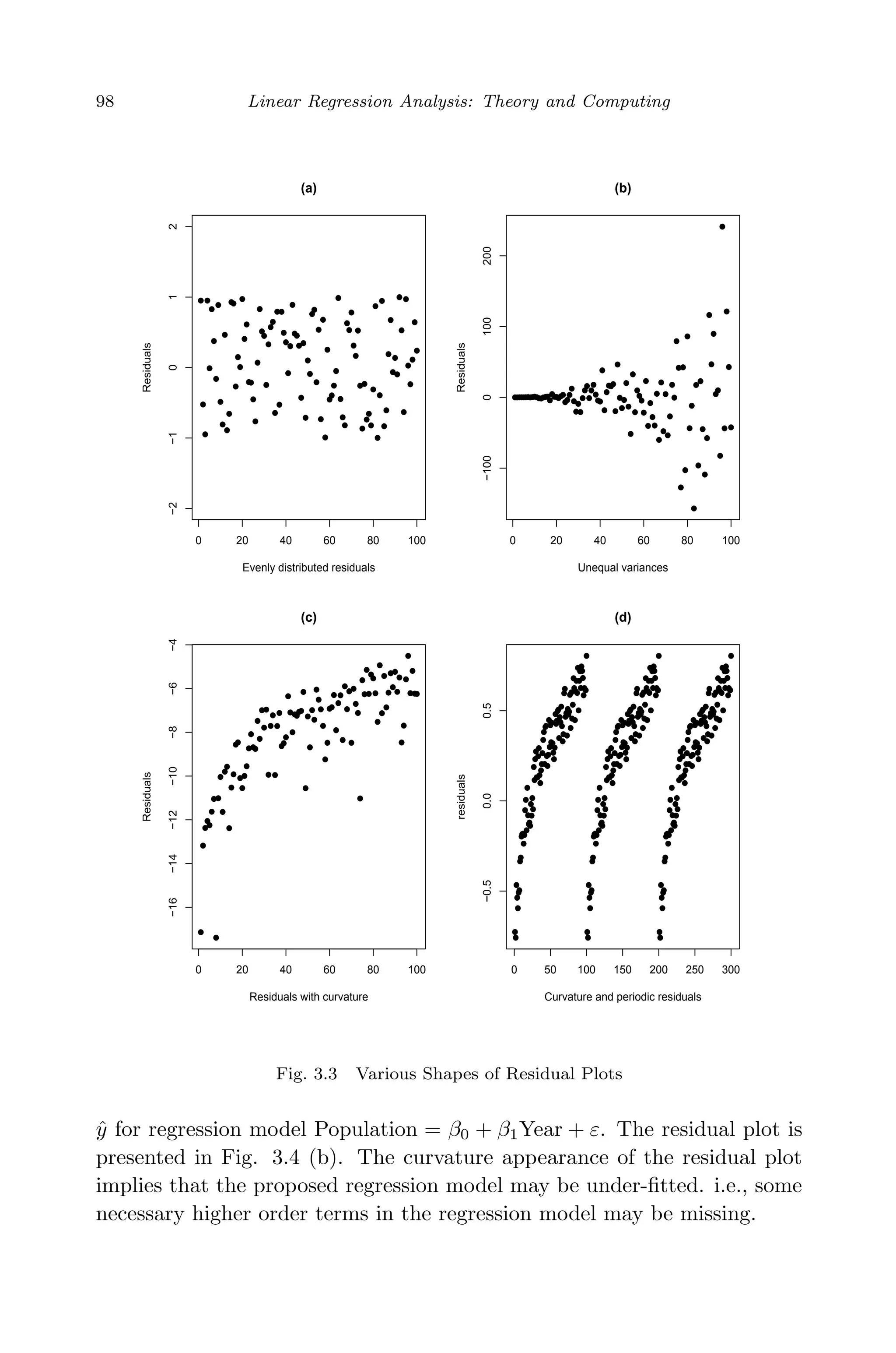
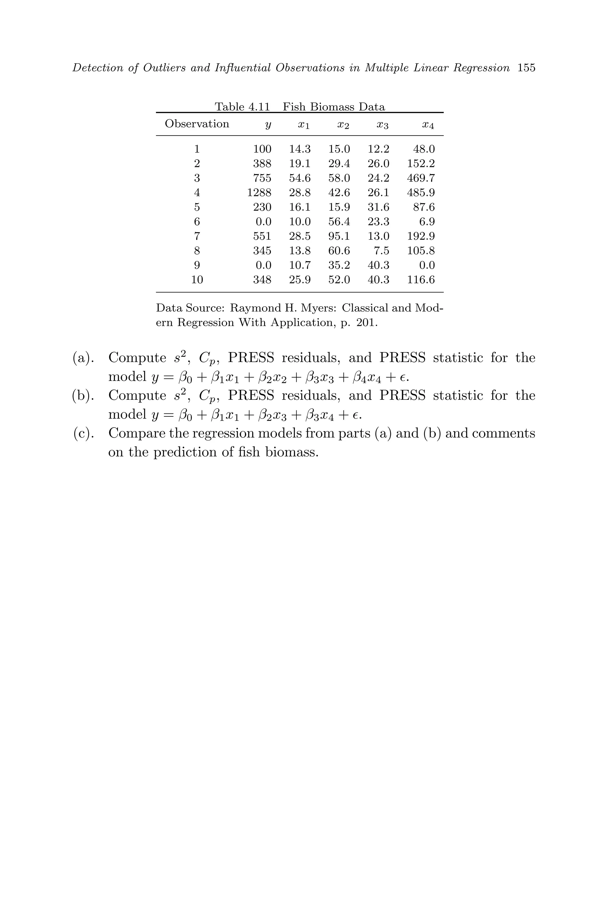
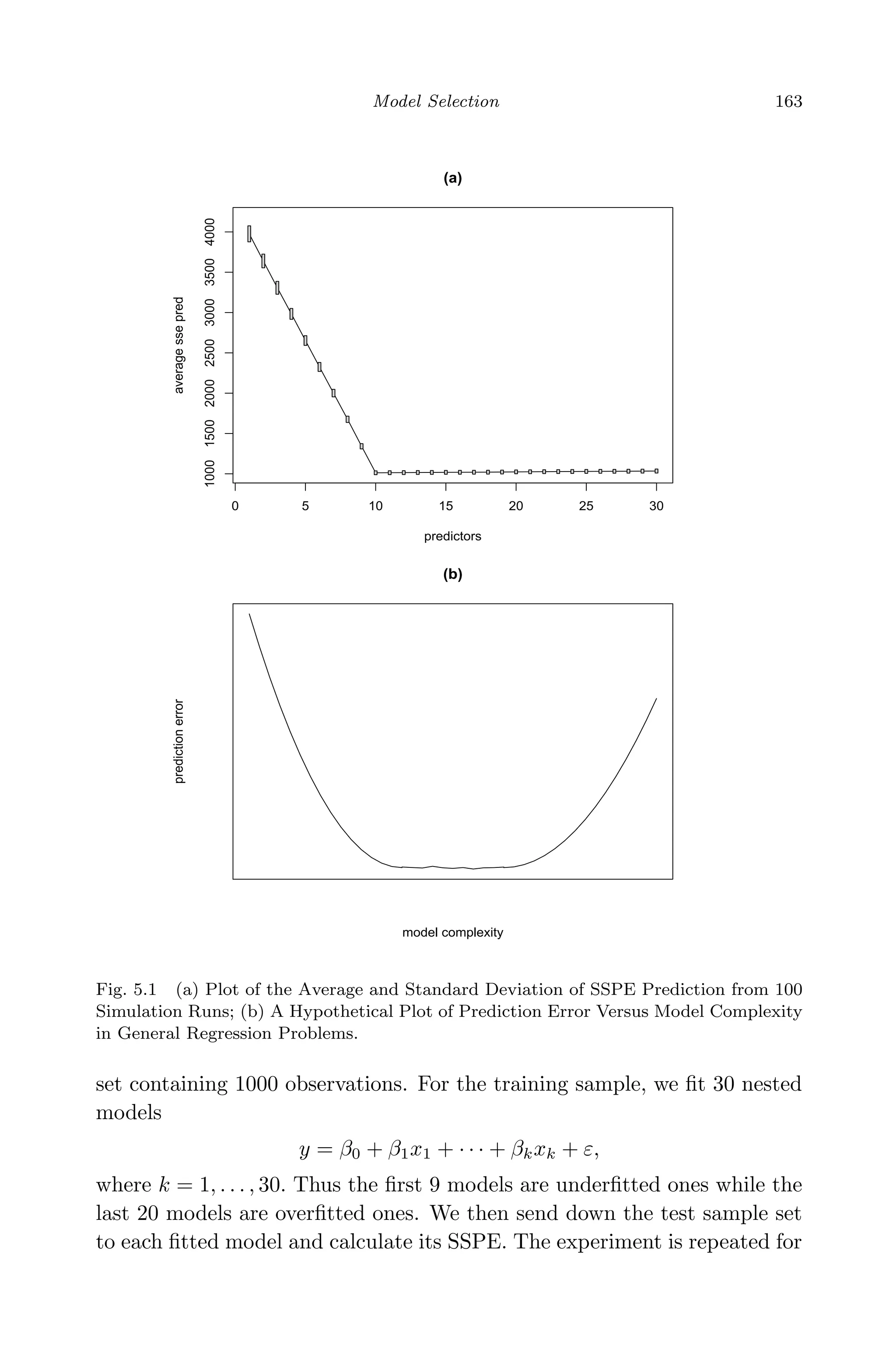
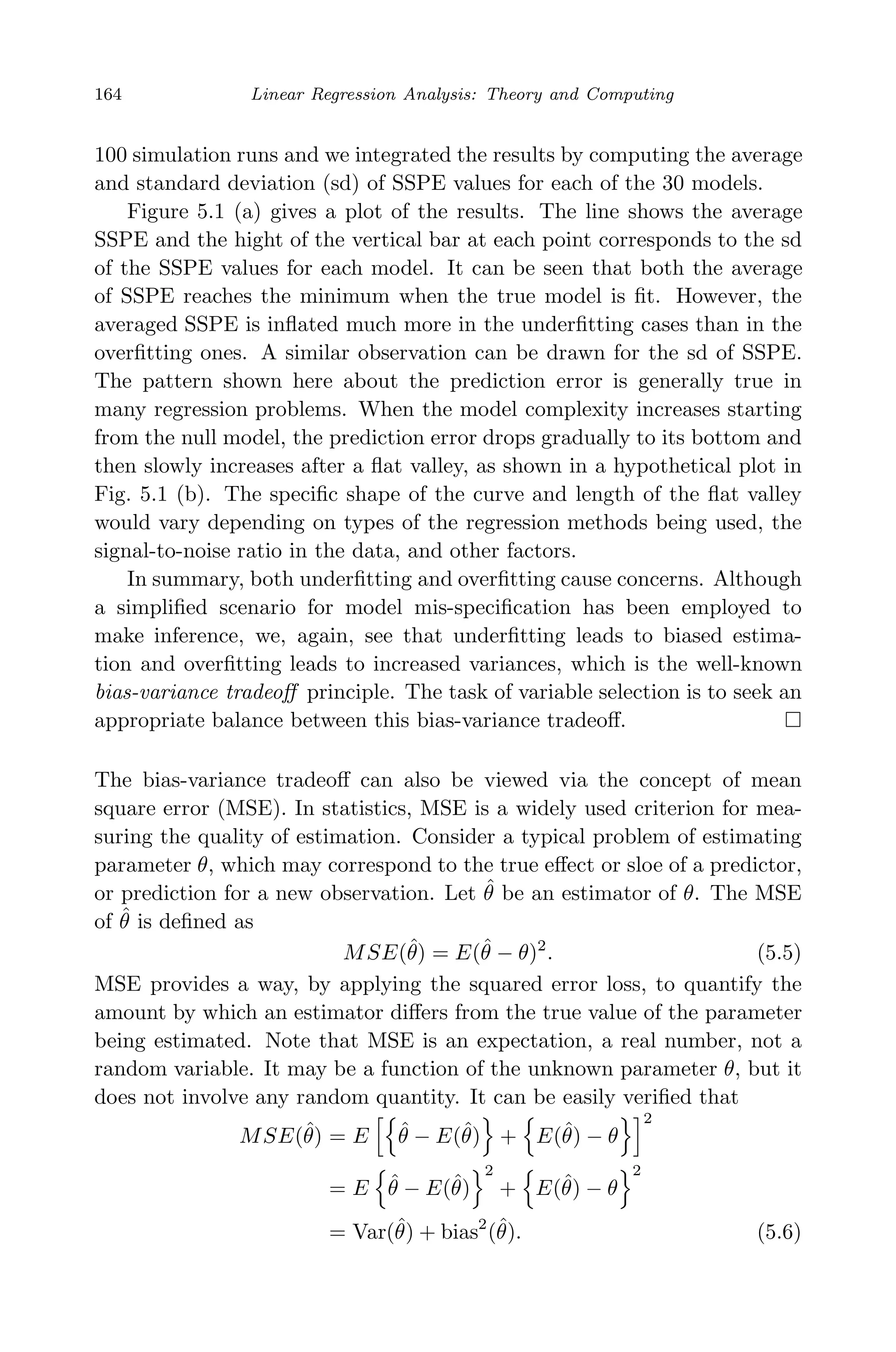
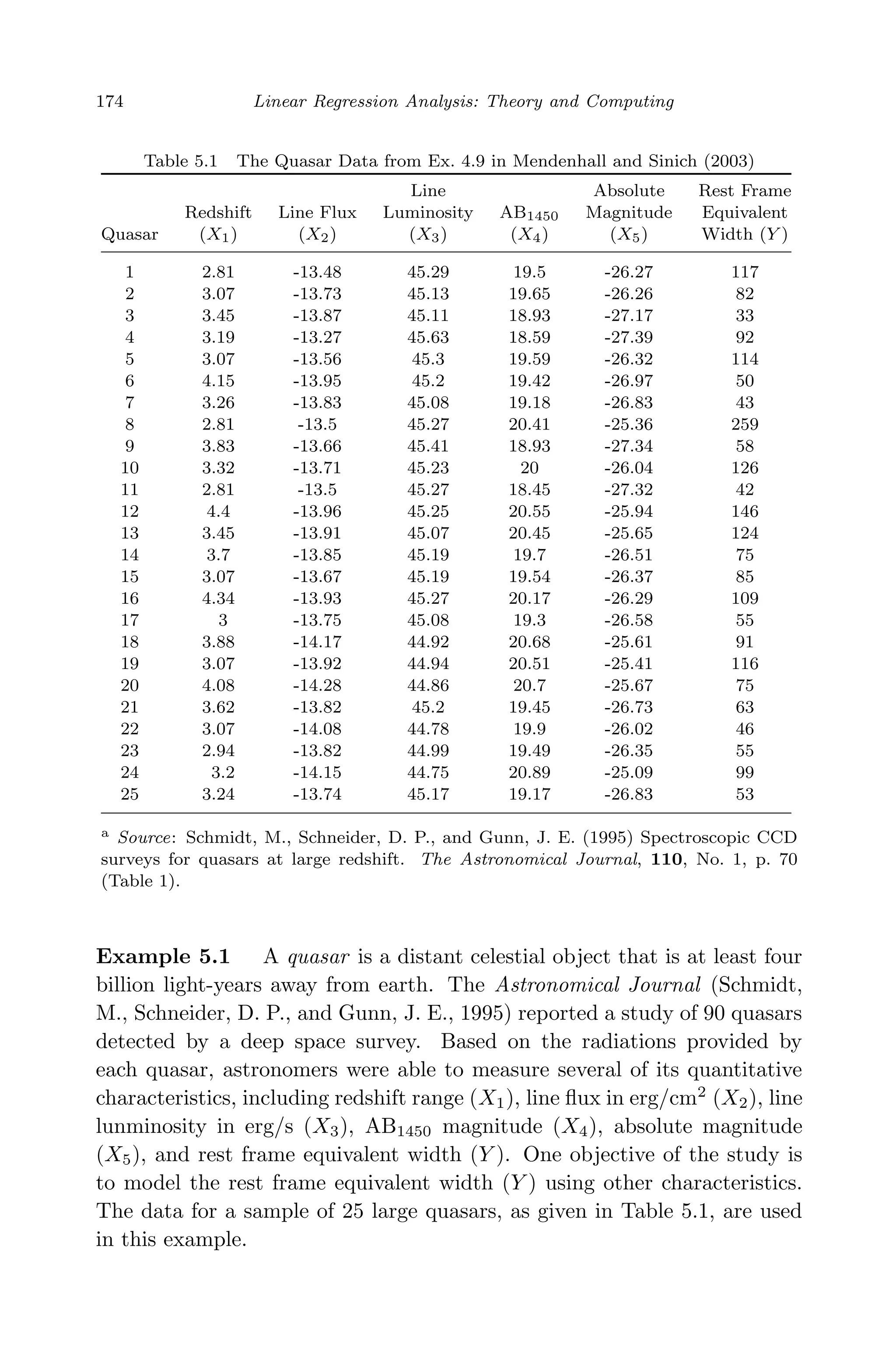
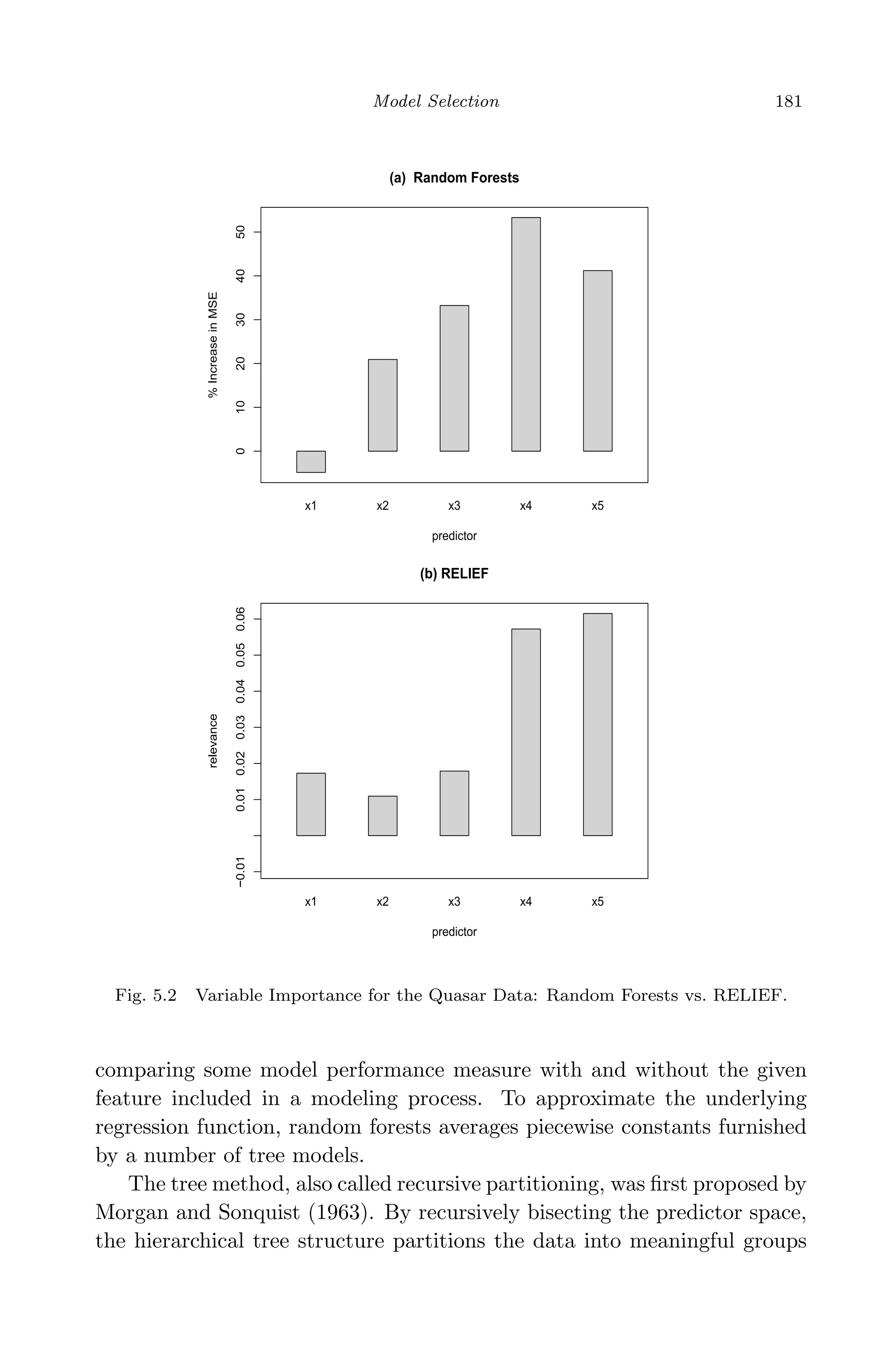
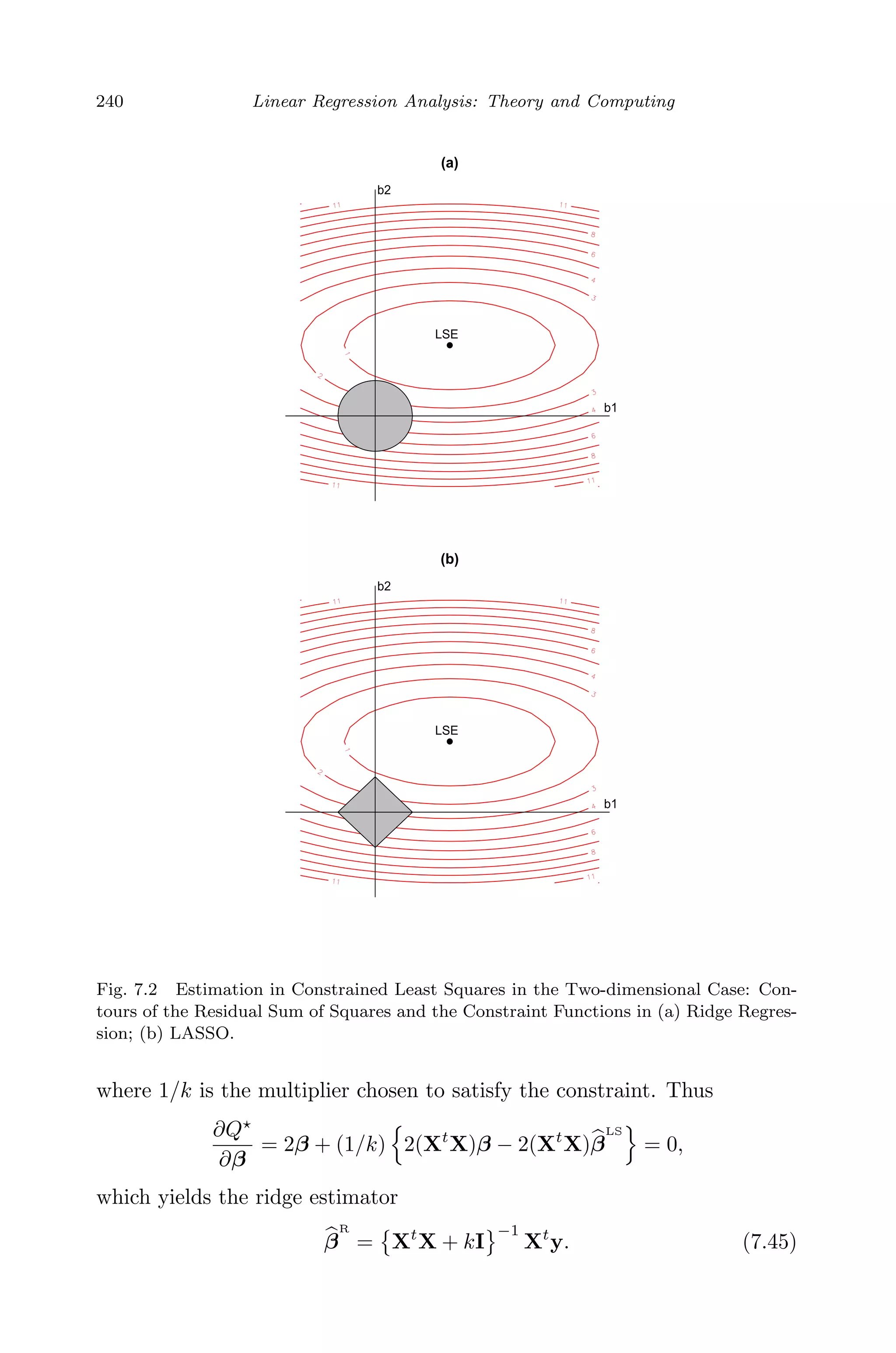
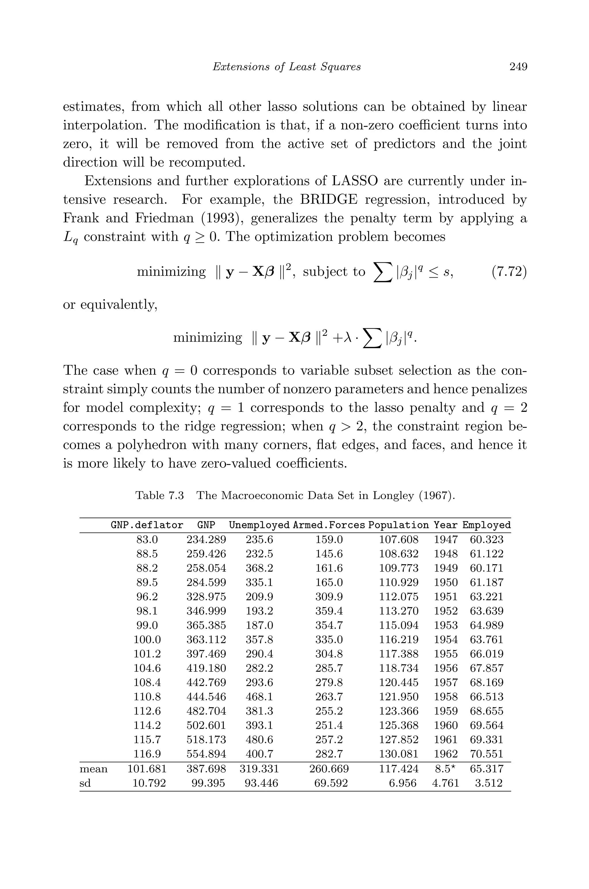
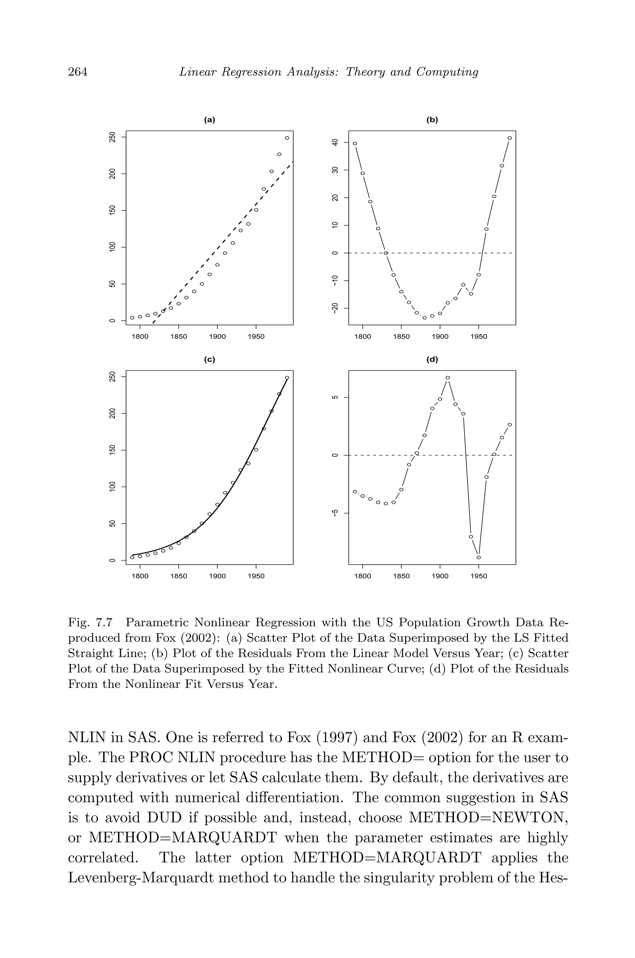
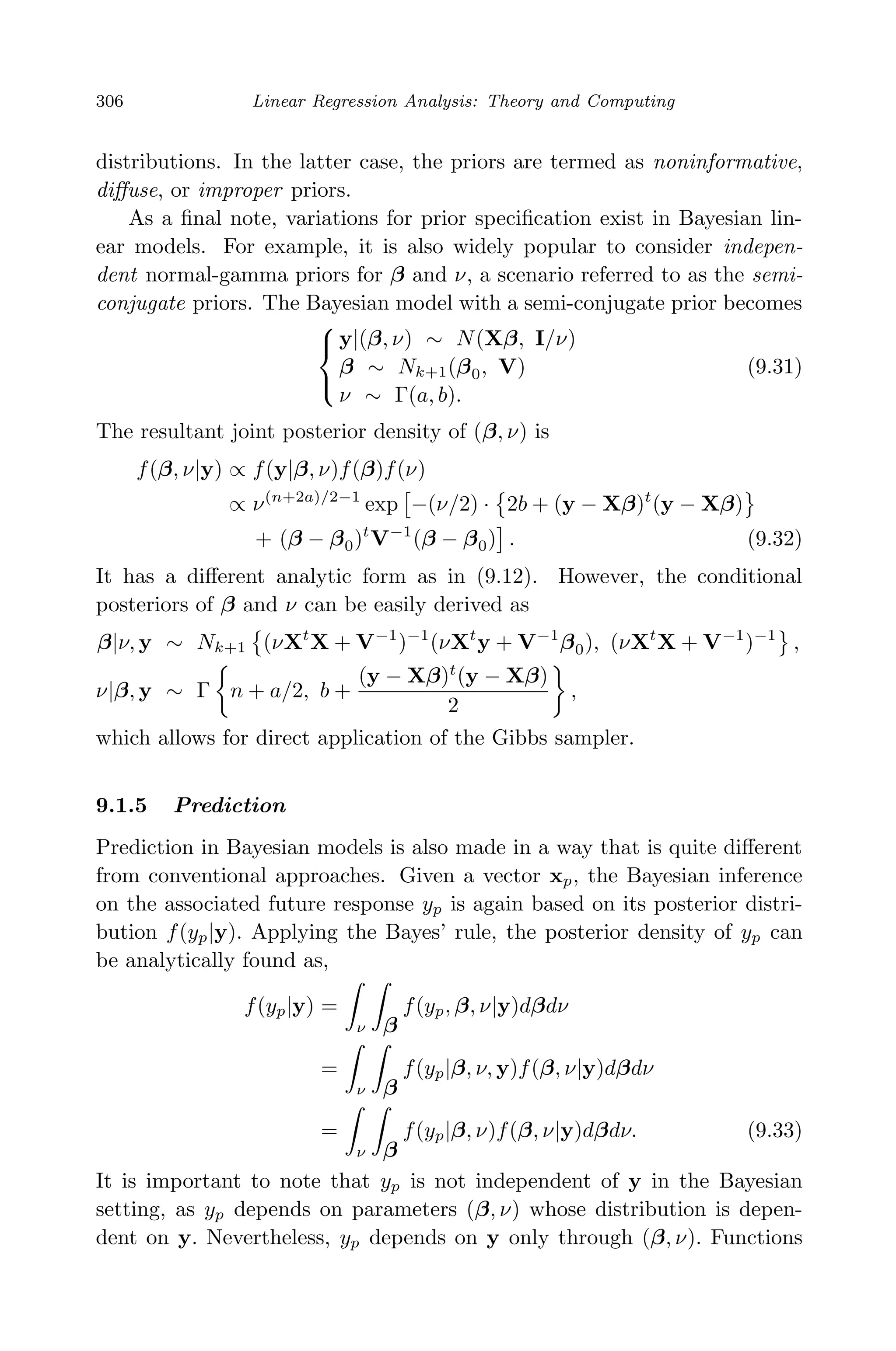
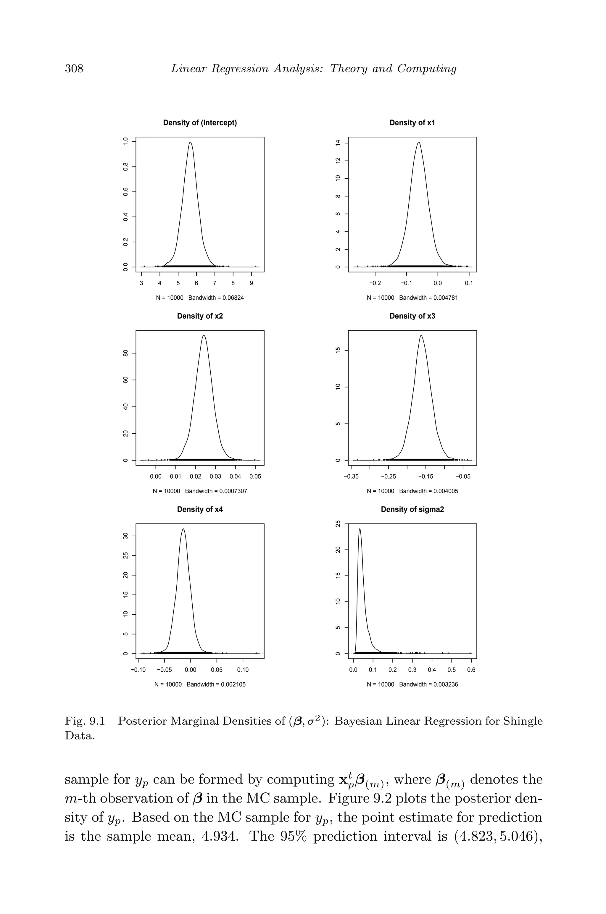
This document provides an overview and summary of linear regression analysis theory and computing. It discusses linear regression models and the goals of regression analysis. It also introduces some key topics that will be covered in the book, including simple and multiple linear regression, model diagnosis, generalized linear models, Bayesian linear regression, and computational methods like least squares estimation. The book aims to serve as a one-semester textbook on fundamental regression analysis concepts for graduate students.


![[DSC Europe 25] Branko Dzakula - From Defense to Attack: How AI Redefines Cyb...](https://cdn.slidesharecdn.com/ss_thumbnails/80bdzdxpr3ky2g0qvyk9-8-251211083048-ce5fc1ee-thumbnail.jpg?width=640&height=640&fit=bounds)
![[DSC Europe 25] Jovan Bogicevic - Legacy to AI-Driven Defense: Transforming D...](https://cdn.slidesharecdn.com/ss_thumbnails/rsarluadt563hntyfc8q-3-251211083849-3e7bc4c0-thumbnail.jpg?width=640&height=640&fit=bounds)


![[DSC Europe 25] Dusan Nesic - Securing Tomorrow’s Infrastructure: Why Cyber-P...](https://cdn.slidesharecdn.com/ss_thumbnails/qikbszfftyowjm2q6duw-1-251211083848-8f2ead6b-thumbnail.jpg?width=640&height=640&fit=bounds)
![[DSC Europe 25] Behzad Hosseini - AI Agents in the Wild: Deploying Models tha...](https://cdn.slidesharecdn.com/ss_thumbnails/3qtejajvsjqrzwfept2c-10-251212103250-7f2b1068-thumbnail.jpg?width=640&height=640&fit=bounds)


![[DSC Europe 25] Katherine Forrest - AI NOW: Understanding the Velocity of Cha...](https://cdn.slidesharecdn.com/ss_thumbnails/wvvbruqfrci0sfq9xwgb-4-251212104007-e5ad1987-thumbnail.jpg?width=640&height=640&fit=bounds)

![[DSC Europe 25] Hans Kleinsman - The Compliance Gearbox: How Tax Tech Mediate...](https://cdn.slidesharecdn.com/ss_thumbnails/dxdytie1toel0hr90bjs-2-251212103250-174fdbe7-thumbnail.jpg?width=640&height=640&fit=bounds)


![[DSC Europe 25] Dunja Adzic Jovanovic - AI and Cybersecurity: Defending Data ...](https://cdn.slidesharecdn.com/ss_thumbnails/o1zylpbhrtwnixxq2xj8-7-251211083048-185086f6-thumbnail.jpg?width=640&height=640&fit=bounds)


![[DSC Europe 25] Jon Dajci - Bridging TradFi and DeFi: Building the Future of ...](https://cdn.slidesharecdn.com/ss_thumbnails/fqmhfvlbqhkihjvqvhmu-7-251211083849-6af7e325-thumbnail.jpg?width=640&height=640&fit=bounds)