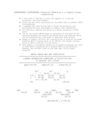
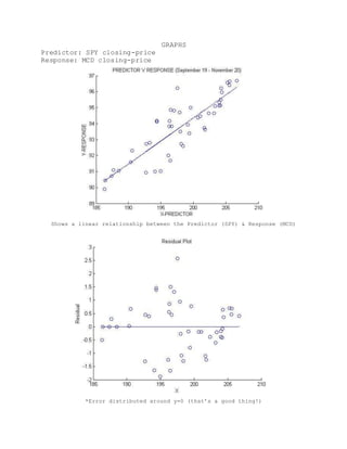
INDEPENDENT COURSEWORK: Financial Modeling & a Simple Linear
Regression
 I took what I learned in class and applied it to my own
interests: the stock market.
 Given the S&P 500’s closing-price, my model aims to predict MCD’s
closing-price.
 I assumed that both stocks had a linear relationship, and
discovered the data and graphs to support that hypothesis.
 R^2 statistic implies SPY price is a decent predictor of MCD
price
 One of the things ANOVA helps to determine is how much of the
variance between the model’s estimated value and observed value
can be accounted for, and helps to quantify those errors.
 Based on today’s (4/3/15) SPY closing price of $206.40, my model
predicts MCD’s closing price to be $96.20. The actual closing
price of MCD is $95.83, a 0.39% error.
 This model is ultimately useless as a predictor because you need
to know SPY’s closing price to predict MCD’s closing price.
However, SPY and MCD close on the same day- Still, great
practice!
ANOVA TABLE AND KEY STATISTICS
===================================================
LINEAR REGRESSION FUNCTION: y^=36.81+00.29x
R squared (%): 74.80
===================================================
xBar=197.80 yBar=93.72 y^Bar=93.72
b0^ b1^ y^
^ : 36.81 00.29
s^2 : 24.82 00.00 00.07
s : 04.98 00.03 00.26
t*: 07.39 11.43
F*: 130.61
SSE SSR SSTO MSE MSR
39.97 118.65 158.62 00.91 118.65
SSE/SSTO SSR/SSTO
00.25 00.75
Xh=206.40 , Y^=96.20
GRAPHS
Predictor: SPY closing-price
Response: MCD closing-price
Shows a linear relationship between the Predictor (SPY) & Response (MCD)
*Error distributed around y=0 (that’s a good thing!)
MATLAB CODE FOR THE LINEAR REGRESSION MODEL:
clc
clear all
%SSR = SUM[(Yhat-Ybar)^2]
%SSE = SUM[(Y-Yhat)^2]
%SSTO = SUM[(Y-Ybar)^2]
%Yhat= B0hat+ B1hat*X
X=importdata('C:/SPYCLOSING.txt');
Y=importdata('C:/MCDCLOSING.txt');
%for i=1:numel(Y)
% X(i)=i;
%end
%X=[rand(1) rand(1) rand(1)];
%Y=[rand(1) rand(1) rand(1)];
%X=transpose(X);
%Y=transpose(Y);
i=0;
for i=1:numel(Y)
T(i)=i+1;
end
clc
fprintf('Last Value: X=%05.2fn', X(numel(X)))
fprintf('Last Value: Y=%05.2fn', Y(numel(Y)))
xPred=input('Predictor Value (X-Level): ');
n=numel(X);
Xbar=0;
Ybar=0;
b1Num=0;
b1Den=0;
for i=1:n
Xbar=Xbar+X(i);
end
for i=1:n
Ybar=Ybar+Y(i);
end
Xbar=Xbar/n;
Ybar=Ybar/n;
%LEAST SQUARES PARAMTER ESTIMATES : b0, b1 and y^
for i=1:n
b1Num=b1Num+((X(i)-Xbar)*(Y(i)-Ybar));
b1Den=b1Den+((X(i)-Xbar)^2);
end
b1=b1Num/b1Den;
b0=Ybar-b1*Xbar;
Yhat=b0+b1.*X;
%SSR
SSR=0;
for i=1:n
SSR=SSR+(Yhat(i)-Ybar)^2;
errBar(i)=Yhat(i)-Ybar;
end
SSR;
%SSE
SSE=0;
for i=1:n
SSE=SSE+(Y(i)-Yhat(i)).^2;
errData(i)=Y(i)-Yhat(i);
end
SSE;
%YHATBAR
sum=0;
for i=1:numel(Yhat)
sum=Yhat(i)+sum;
end
yHatBar=sum/numel(Yhat);
%SSTO
SSTO=SSE+SSR;
Rsquared=SSR/SSTO;
%MSE = s^2 = Sample Variance
MSE=SSE/(n-2); %2 degrees of freedom are lost in estimating b0
and b1
rootMSE=sqrt(MSE);
%MSR
MSR=SSR/1;
%s^2[YHath]
x=0;
Xh=xPred; %X Level
for i=1:n
x=(X(i)-Xbar).^2 + x;
end
sSquaredYh=MSE*( (1/n)+ ((Xh-Xbar).^2)/x);
sYhatH=sqrt(sSquaredYh);
yhatH=b0+b1*Xh;
%s^2[b0]
Ssquaredb0=0;
Ssquaredb0=MSE*((1/n)+ (Xbar^2)/(x));
sB0=sqrt(Ssquaredb0);
%s^2[b1]
varianceb1=1;
Ssquaredb1=MSE/(x);
sB1=sqrt(Ssquaredb1);
%MATRIX FORM
XM=ones(numel(X), 1);
XM=[XM zeros(size(XM,1),1)];
for i=1:n
XM(i,2)=X(i);
end
XM;
YM=Y;
XMtrans=transpose(XM);
XtransposeTimesX=XMtrans*XM;
XtransposeTimesY=XMtrans*YM;
InverseXXt=inv(XtransposeTimesX);
BETA=InverseXXt*XtransposeTimesY;
YhatM=XM*BETA;
ResidualM=YM-YhatM;
VarCov=MSE*InverseXXt;
%t statistic
tb1=b1/sB1;
tb0=b0/sB0;
%f statstic
F=MSR/MSE;
clc
%fprintf('X t t Y t t t Y^ ttn')
%for i =1:numel(X)
%fprintf('%05.2f t %05.2f t %05.2fn', X(i), Y(i), Yhat(i) )
%end
fprintf('n')
fprintf('===================================================n')
fprintf('LINEAR REGRESSION FUNCTION: y^=%05.2f+%05.2fxn',b0,b1
)
fprintf('R squared (%%): %05.2f n', Rsquared*100)
fprintf('===================================================')
fprintf('n')
fprintf('xBar=%05.2f t yBar=%05.2f t y^Bar=%05.2fn', Xbar,
Ybar, yHatBar)
fprintf('nn')
fprintf('t b0^ t t b1^ t t y^n')
fprintf('^ : %05.2f t %05.2fn',BETA(1), BETA(2))
fprintf('s^2 : %05.2f t %05.2f %05.2fn', Ssquaredb0,
Ssquaredb1, sSquaredYh)
fprintf('s : %05.2f t %05.2f %05.2fn', sB0, sB1,
sqrt(sSquaredYh))
fprintf('t* : %05.2f t %05.2f n', tb0, tb1)
fprintf('F* : ttttt %05.2f n', F)
fprintf('nnn')
%fprintf('Y-Y^ ttt Y^-Ybarn')
%for i=1:numel(X)
%fprintf('%05.2f t tt%05.2fn', errData(i), errBar(i))
%end
fprintf('SSE tt SSR tt SSTO t MSE t MSRn')
fprintf('%05.2f t %05.2f t %05.2f t %05.2f t %05.2fn', SSE,
SSR, SSTO, MSE, MSR)
fprintf('tttSSE/SSTO tt SSR/SSTOn')
fprintf('ttt%05.2f ttt %05.2fn', SSE/SSTO, SSR/SSTO)
prediction=b0+b1*xPred;
figure(1)
%Residual plot
scatter(X, ResidualM)
hold on
for i=1:n
why(i)=0;;
end
plot(X,why)
xlabel('X')
ylabel('Residual')
title('Residual Plot')
figure(2)
scatter(X,Y)
hold on
plot(X,Yhat)
title('PREDICTOR V RESPONSE (September 19 - November 20)')
xlabel('X-PREDICTOR')
ylabel('Y-RESPONSE')
figure(3)
plot(T,Y)
xlabel('n')
ylabel('Response')
title('Response v Time')
figure (4)
plot(T,X)
xlabel('n')
ylabel('Predictor')
title('Predictor v Time')
fprintf('nttttXh=%05.2f , Y^=%05.2fn', xPred, prediction)
fprintf('n')

Financialmodeling

  • 1.
    INDEPENDENT COURSEWORK: FinancialModeling & a Simple Linear Regression  I took what I learned in class and applied it to my own interests: the stock market.  Given the S&P 500’s closing-price, my model aims to predict MCD’s closing-price.  I assumed that both stocks had a linear relationship, and discovered the data and graphs to support that hypothesis.  R^2 statistic implies SPY price is a decent predictor of MCD price  One of the things ANOVA helps to determine is how much of the variance between the model’s estimated value and observed value can be accounted for, and helps to quantify those errors.  Based on today’s (4/3/15) SPY closing price of $206.40, my model predicts MCD’s closing price to be $96.20. The actual closing price of MCD is $95.83, a 0.39% error.  This model is ultimately useless as a predictor because you need to know SPY’s closing price to predict MCD’s closing price. However, SPY and MCD close on the same day- Still, great practice! ANOVA TABLE AND KEY STATISTICS =================================================== LINEAR REGRESSION FUNCTION: y^=36.81+00.29x R squared (%): 74.80 =================================================== xBar=197.80 yBar=93.72 y^Bar=93.72 b0^ b1^ y^ ^ : 36.81 00.29 s^2 : 24.82 00.00 00.07 s : 04.98 00.03 00.26 t*: 07.39 11.43 F*: 130.61 SSE SSR SSTO MSE MSR 39.97 118.65 158.62 00.91 118.65 SSE/SSTO SSR/SSTO 00.25 00.75 Xh=206.40 , Y^=96.20
  • 2.
    GRAPHS Predictor: SPY closing-price Response:MCD closing-price Shows a linear relationship between the Predictor (SPY) & Response (MCD) *Error distributed around y=0 (that’s a good thing!)
  • 4.
    MATLAB CODE FORTHE LINEAR REGRESSION MODEL: clc clear all %SSR = SUM[(Yhat-Ybar)^2] %SSE = SUM[(Y-Yhat)^2] %SSTO = SUM[(Y-Ybar)^2] %Yhat= B0hat+ B1hat*X X=importdata('C:/SPYCLOSING.txt'); Y=importdata('C:/MCDCLOSING.txt'); %for i=1:numel(Y) % X(i)=i; %end %X=[rand(1) rand(1) rand(1)]; %Y=[rand(1) rand(1) rand(1)]; %X=transpose(X); %Y=transpose(Y); i=0; for i=1:numel(Y) T(i)=i+1; end clc fprintf('Last Value: X=%05.2fn', X(numel(X))) fprintf('Last Value: Y=%05.2fn', Y(numel(Y))) xPred=input('Predictor Value (X-Level): '); n=numel(X); Xbar=0; Ybar=0; b1Num=0; b1Den=0; for i=1:n Xbar=Xbar+X(i); end for i=1:n Ybar=Ybar+Y(i); end Xbar=Xbar/n; Ybar=Ybar/n;
  • 5.
    %LEAST SQUARES PARAMTERESTIMATES : b0, b1 and y^ for i=1:n b1Num=b1Num+((X(i)-Xbar)*(Y(i)-Ybar)); b1Den=b1Den+((X(i)-Xbar)^2); end b1=b1Num/b1Den; b0=Ybar-b1*Xbar; Yhat=b0+b1.*X; %SSR SSR=0; for i=1:n SSR=SSR+(Yhat(i)-Ybar)^2; errBar(i)=Yhat(i)-Ybar; end SSR; %SSE SSE=0; for i=1:n SSE=SSE+(Y(i)-Yhat(i)).^2; errData(i)=Y(i)-Yhat(i); end SSE; %YHATBAR sum=0; for i=1:numel(Yhat) sum=Yhat(i)+sum; end yHatBar=sum/numel(Yhat); %SSTO SSTO=SSE+SSR; Rsquared=SSR/SSTO; %MSE = s^2 = Sample Variance MSE=SSE/(n-2); %2 degrees of freedom are lost in estimating b0 and b1 rootMSE=sqrt(MSE); %MSR MSR=SSR/1; %s^2[YHath] x=0;
  • 6.
    Xh=xPred; %X Level fori=1:n x=(X(i)-Xbar).^2 + x; end sSquaredYh=MSE*( (1/n)+ ((Xh-Xbar).^2)/x); sYhatH=sqrt(sSquaredYh); yhatH=b0+b1*Xh; %s^2[b0] Ssquaredb0=0; Ssquaredb0=MSE*((1/n)+ (Xbar^2)/(x)); sB0=sqrt(Ssquaredb0); %s^2[b1] varianceb1=1; Ssquaredb1=MSE/(x); sB1=sqrt(Ssquaredb1); %MATRIX FORM XM=ones(numel(X), 1); XM=[XM zeros(size(XM,1),1)]; for i=1:n XM(i,2)=X(i); end XM; YM=Y; XMtrans=transpose(XM); XtransposeTimesX=XMtrans*XM; XtransposeTimesY=XMtrans*YM; InverseXXt=inv(XtransposeTimesX); BETA=InverseXXt*XtransposeTimesY; YhatM=XM*BETA; ResidualM=YM-YhatM; VarCov=MSE*InverseXXt; %t statistic tb1=b1/sB1; tb0=b0/sB0; %f statstic F=MSR/MSE; clc
  • 7.
    %fprintf('X t tY t t t Y^ ttn') %for i =1:numel(X) %fprintf('%05.2f t %05.2f t %05.2fn', X(i), Y(i), Yhat(i) ) %end fprintf('n') fprintf('===================================================n') fprintf('LINEAR REGRESSION FUNCTION: y^=%05.2f+%05.2fxn',b0,b1 ) fprintf('R squared (%%): %05.2f n', Rsquared*100) fprintf('===================================================') fprintf('n') fprintf('xBar=%05.2f t yBar=%05.2f t y^Bar=%05.2fn', Xbar, Ybar, yHatBar) fprintf('nn') fprintf('t b0^ t t b1^ t t y^n') fprintf('^ : %05.2f t %05.2fn',BETA(1), BETA(2)) fprintf('s^2 : %05.2f t %05.2f %05.2fn', Ssquaredb0, Ssquaredb1, sSquaredYh) fprintf('s : %05.2f t %05.2f %05.2fn', sB0, sB1, sqrt(sSquaredYh)) fprintf('t* : %05.2f t %05.2f n', tb0, tb1) fprintf('F* : ttttt %05.2f n', F) fprintf('nnn') %fprintf('Y-Y^ ttt Y^-Ybarn') %for i=1:numel(X) %fprintf('%05.2f t tt%05.2fn', errData(i), errBar(i)) %end fprintf('SSE tt SSR tt SSTO t MSE t MSRn') fprintf('%05.2f t %05.2f t %05.2f t %05.2f t %05.2fn', SSE, SSR, SSTO, MSE, MSR) fprintf('tttSSE/SSTO tt SSR/SSTOn') fprintf('ttt%05.2f ttt %05.2fn', SSE/SSTO, SSR/SSTO) prediction=b0+b1*xPred; figure(1) %Residual plot scatter(X, ResidualM) hold on
  • 8.
    for i=1:n why(i)=0;; end plot(X,why) xlabel('X') ylabel('Residual') title('Residual Plot') figure(2) scatter(X,Y) holdon plot(X,Yhat) title('PREDICTOR V RESPONSE (September 19 - November 20)') xlabel('X-PREDICTOR') ylabel('Y-RESPONSE') figure(3) plot(T,Y) xlabel('n') ylabel('Response') title('Response v Time') figure (4) plot(T,X) xlabel('n') ylabel('Predictor') title('Predictor v Time') fprintf('nttttXh=%05.2f , Y^=%05.2fn', xPred, prediction) fprintf('n')