Downloaded 26 times


![“Perhaps the most widely used (and misused) multivariate
[technique] is factor analysis. Few statisticians are neutral about
this technique. Proponents feel that factor analysis is the
greatest invention since the double bed, while its detractors feel
it is a useless procedure that can be used to support nearly any
desired interpretation of the data. The truth, as is usually the case,
lies somewhere in between. Used properly, factor analysis can
yield much useful information; when applied blindly, without
regard for its limitations, it is about as useful and informative as
Tarot cards. In particular, factor analysis can be used to explore
the data for patterns, confirm our hypotheses, or reduce the
Many variables to a more manageable number.
-- Norman Streiner, PDQ Statistics](https://image.slidesharecdn.com/factoranalysis-141225131131-conversion-gate01/85/Factor-analysis-9-320.jpg)
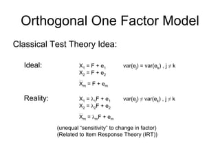
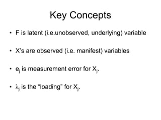
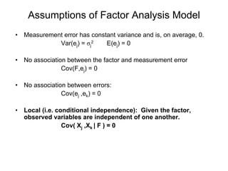
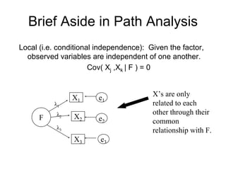
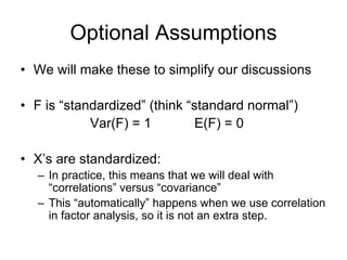
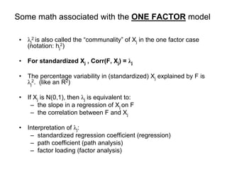
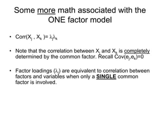
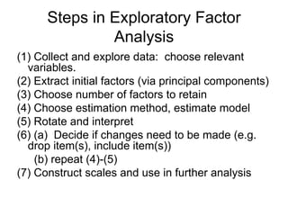
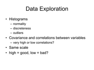
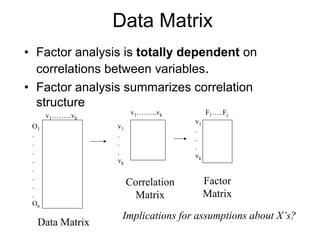
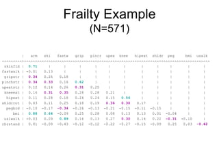
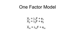
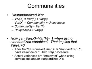
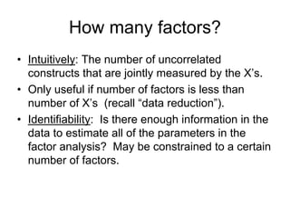
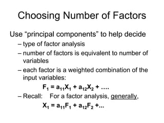
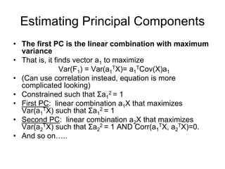

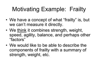
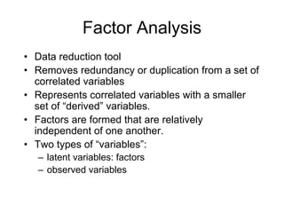
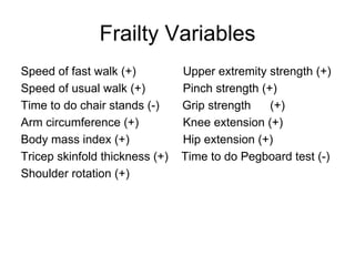
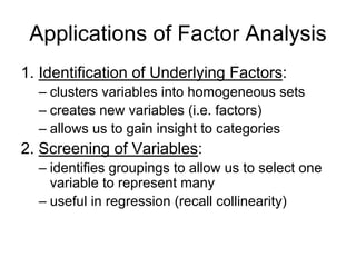
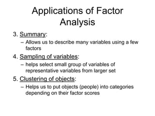
This document discusses factor analysis, a statistical technique used to reduce the dimensionality of correlated variables into a smaller number of underlying factors. It begins by motivating factor analysis through an example involving measuring frailty. It then provides an overview of factor analysis, including key concepts like observed and latent variables, assumptions of the factor model, and common applications. The document also covers the mathematical underpinnings of one-factor and multiple-factor models, and explains important outputs of factor analysis like factor loadings and communalities.