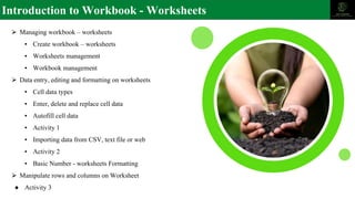
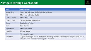
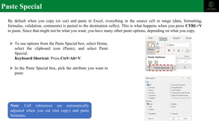
This document provides an overview of managing worksheets in Excel. It discusses how to create and manage workbooks and worksheets, enter and format cell data, and manipulate rows and columns. The document covers topics such as creating and renaming worksheets, adding and deleting sheets, navigating between sheets, moving and copying sheets, and saving workbooks. It also discusses selecting cells and ranges, copying and pasting data, commenting on cells, and deleting or replacing cell content.

1. Introduction to Workbook - Worksheets
⮚ Managing workbook – worksheets
▪ Create workbook – worksheets
▪ Worksheets management
▪ Workbook management
⮚ Data entry, editing and formatting on worksheets
▪ Cell data types
▪ Enter, delete and replace cell data
▪ Autofill cell data
▪ Activity 1
▪ Importing data from CSV, text file or web
▪ Activity 2
▪ Basic Number - worksheets Formatting
⮚ Manipulate rows and columns on Worksheet
● Activity 3

2. Create Workbook and Worksheets
To create a Workbook:
⮚ Open Excel
⮚ Select Blank workbook. (Or press Ctrl + N).
Note: when you click on Blank workbook, one
worksheet will automatically added and named
Sheet1.

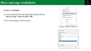
3. Change the name and color of worksheets
By default, Excel names worksheets Sheet1, Sheet2, Sheet3 and so on, but you can easily rename them.
There are 3 ways to rename a worksheet:
⮚ Double-click the sheet tab, and type the new name.
⮚ Right-click the sheet tab, click Rename, and type the
new name.
⮚ Use the keyboard shortcut Alt+H > O > R, and type
the new name.
To change the color of a worksheet:
⮚ Right-click the sheet tab, click Tab color, and the
color
Important: Worksheet names cannot:
• Be blank .
• Contain more than 31 characters.
• Contain any of the following characters: / ? * : [ ]
• Begin or end with an apostrophe ('), but they can be used in between text or numbers in a name.
• Be named "History". This is a reserved word Excel uses internally.

4. Add, delete, hide and unhide worksheets
In Excel, you can easily add, delete, hide and unhide worksheets in your
workbook.
Add a worksheet:
⮚ Select the New Sheet at the
bottom of the workbook.
⮚ Or, select Home > Insert > Insert
Sheet.
Delete a worksheet
⮚ Right-click the Sheet tab and select
Delete.
⮚ Or, select the sheet, and then select
Home > Delete > Delete Sheet.
Hide/Unhide a worksheet
⮚ Right-click the Sheet tab and
select Hide/Unhide
Attention: there is no undo for a
deleted worksheet unless the workbook
is not saved

5. Navigate through worksheets
To change the active cell
⮚ Use the Mouse to select the cell
⮚ Use the scrollbar the show the hidden cells
⮚ Use the Arrow Keys to move the active cell
⮚ Use “PageUp/ Down Keys respectively
To move from one worksheet to another in Excel
⮚ Click on the worksheet name
⮚ Use the shortcut “Ctrl” + “PageUp” to move to the previous Worksheet
⮚ Use the shortcut “Ctrl” + “PageDown” to move to the next Worksheet
⮚ Use Page down (Fn + Down Arrow), Page Up (Fn + Up Arrow)

6. Navigate through worksheets
Keys Descriptions
Arrow Keys Move one cell to the Right, Left, Up or Down
Tab Move one cell to the Right
CTRL + Home Move the A1 cell
CTRL + End To end of typed information
Home Beginning of a line
End End of a line
Page Down Down one screen
Page Up Up one screen
F5 To a specific page
Scroll bars Appear at the right and on the bottom. You may click the scroll arrows, drag the scroll box or,
click the scroll bar to move through the document

7. Move and copy worksheets
To move a worksheet:
⮚ To move the tab to the end, right-click the Sheet tab then
Move or Copy > (move to end) > OK .
⮚ Or, click and drag to tab to any spot.

8. Save, save as, open Workbooks
⮚ Wherever you want to save your workbook (on your computer or the web, for example), you do all your saving on
the File tab.
⮚ While you’ll use Save (or press Ctrl + S) to save an existing workbook in its current location, you need to use
Save As to save your workbook for the first time, in a different location, or to create a copy of your workbook in
the same or another location.
• Click File > Save As.
• Under Save As, pick the place where you want to save your workbook.
• Choose a Location option
• Click Browse to find the location you want in your Documents folder.
• To pick another location on your computer, click Desktop, and then pick
the exact place where you want to save your workbook.
• In the File name box, enter a name for a new workbook. Enter a
different name if you’re creating a copy of an existing workbook.
• Save As dialog box
• To save your workbook in a different file format (like .xls or .txt), in the
Save as type list (under the File name box), pick the format you want.
• Click Save.

9. Cell data types
Text Number
Dates
Formulas Errors
Images

10. Cell Address Nomenclature
A cell address refers to a cell or a range of cells on a worksheet and can be used in
a formula so that Excel can find the values or data that you want that formula to
calculate.
In one or several formulas, you can use a cell address to refer to:
❖ Data from one or more contiguous cells on the worksheet.
❖ Data contained in different areas of a worksheet.
❖ Data on other worksheets in the same workbook.
For Example:
Formula Refers To
=B4 The value in cell B4.
=B5:D11 The value in all cells B5 through D11
=Sheet2!A7 Cell A7 on Sheet2
=Tmax-Tmin The cells named Tmax and Tmin
Note: the address of a
selected cell is shown in the
name box

11. Enter cell data
⮚ To enter data in any cell, just select the cell and start typing.
⮚ To move to the cell below, press ENTER
⮚ In case you are entering dates, enter it in a format that Excel
recognizes as a date (such as 01-01-2023 or 01 Jan 2023 or
01/01/2023).
Note: By default
⮚ Text are aligned on the left
⮚ Numbers, Dates are aligned on the right
⮚ Errors are aligned on the center

12. Selecting Cells and Ranges
⮚ To select contiguous cells, click on one cell, hold left-click then drag to select cells
⮚ You can quickly locate and select specific cells or ranges by entering their names or
cell references in the Name box, which is located to the left of the formula bar:
⮚ You can also select named or unnamed cells or ranges by using the Go To (F5 or
Ctrl + G) command.
⮚ Select non-contiguous cells or ranges: Hold down the Ctrl key, and left-click each
cell or range you want to include. If you over select, you can click on the unintended
cell to de-select it.
Important: To select named cells and
ranges, you need to define them
first.

13. Copying and Moving Cells and Ranges
Copy cells by using Copy and Paste:
⮚ Select the cell or range of cells.
⮚ Select Copy or press Ctrl + C.
⮚ Select Paste or press Ctrl + V.
Move cells by drag and dropping:
⮚ Select the cells or range of cells that you want to move or copy.
⮚ Point to the border of the selection.
⮚ When the pointer becomes a move pointer, drag the cell or range of
cells to another location.
Move cells by using Cut and Paste:
⮚ Select a cell or a cell range.
⮚ Select Home > Cut or press Ctrl + X.
⮚ Select a cell where you want to move the data.
⮚ Select Home > Paste or press Ctrl + V.
Note: when you move or copy a cell, Excel
moves or copies the cell, including formulas
and their resulting values, cell formats, and
comments.

14. Paste Special
By default when you copy (or cut) and paste in Excel, everything in the source cell or range (data, formatting,
formulas, validation, comments) is pasted to the destination cell(s). This is what happens when you press CTRL+V
to paste. Since that might not be what you want, you have many other paste options, depending on what you copy.
⮚ To use options from the Paste Special box, select Home,
select the clipboard icon (Paste), and select Paste
Special.
Keyboard Shortcut: Press Ctrl+Alt+V.
⮚ In the Paste Special box, pick the attribute you want to
paste
Note: Cell references are automatically
adjusted when you cut (not copy) and paste
formulas.

15. Select Special Cells (Go to Special)
To quickly find and select all cells that contain specific types of data or only cells that meet specific, click Special in
the Go To popup window, and then click the option that you want.
Select named or unnamed cells or ranges by using the Go
To command:
⮚ Press F5 or CTRL+G to launch the Go To dialog.
⮚ In the Go To list, click the name of the cell or range that
you want to select, or type the cell reference in the
Reference box, then press OK.

16. Using Find and Replace to Select Cells
Use the Find and Replace features in Excel to search for something in your workbook, such as a particular number or
text string. You can either locate the search item for reference, or you can replace it with something else. You can
include wildcard characters such as question marks, tildes, and asterisks, or numbers in your search terms. You can
search by rows and columns, search within comments or values, and search within worksheets or entire workbooks.
⮚ Replace: To replace text or numbers, press Ctrl+H,
or go to Home > Editing > Find & Select > Replace
⮚ Find: To find something, press Ctrl+F, or
go to Home > Editing > Find & Select >
Find.

17. Adding Comments
In Excel for Microsoft 365, you can use Comments to have conversations with others and they can reply to continue
the discussion. You can add comments to cells. When a cell has a comment, an indicator appears in the corner of the
cell. When you hover your cursor over the cell, the comment appears.
Add a comment to start a conversation:
⮚ Right-click a cell and select Insert Comment.
⮚ Enter your comment and select Post.
Edit a comment:
⮚ Hover over the cell, hover over the comment, and select
Edit.
Resolve a comment:
⮚ Hover over the cell, hover over the comment, and select
... More Actions.
⮚ Select Resolve thread.
Delete a comment:
⮚ Right-click the cell and select Delete Comment.

18. Delete cell data
The simple way to delete data of multiple cells is to
⮚ press “DELETE”
⮚ right-click in the cell, then select Delete
⮚ go to HOME, Option Editing then Clear

19. Replace cell data
To replace a data of a cell (AI) by the data in another
cell (AJ) by
⮚ Go to cell (AJ)
⮚ Use you mouse to hold the border of cell (AJ)
⮚ Drag or drop it on cell (AI)
Note that
▪ the data in cell (AJ) is deleted
▪ The data and its format is moved to cell (AI)
If you wish to keep the data of (Aj), you can use the
copy (CTRL + C) and paste (CTRL + V) option.
This gives you more flexibility with type of paste
This gives you more flexibility with type of paste

20. Autofill cell data
Click and hold the left mouse button, and drag the
plus sign over the cells you want to fill
Icon fill option (image) gives additional control on the
autofill

21. Autofill cell data
Create this excel file with the active
Cell on B2
Use “SHIFT + Down Arrow” to select
the cell B2 and B3
Drag the plus sign up to the cell B13
What do you notice from Jan to Dec?

22. Activity1
1. Create an empty workbook named Activity 1
2. Name your worksheet Activity 1
3. Enter the date, year, month day, T_min and Tmax values as
presented in the image for the three first Rows
4. Auto fill the value of Columns A, B, C and D
5. Complete others values in Columns E and F
6. What is written at A5, E6 and F3
7. Save your Excel file in your desired folder
8. Create new columns G1:G8
9. Customize the cells all border, font size =12; Middle and Left
Align, first Row angle counterclockwise orientation
10. Name cell G1 as T_mean
11. Calculate the average temperature in cell G2 using the formula
“= 0.5*(E2+F2)”
12. Use the formula in G2 to autofill the remain cells from G3 to
G8

23. Importing data from CSV/Text
To get started:
⮚ Click on Data Tab
⮚ Choose a CSV/Text file
⮚ The Import Data window appears in which one
can specify:
❖ File Origin
❖ Delimiter
❖ Data Type Detection
CSV stands for Comma Separated Values, is a widely common
file format of data. In which the columns are separated by a
delimiter in a standard text file.
Alternative: Use the File-Open menu and select the
file. Make sure to display all file types otherwise a
txt/csv file will not be visible.

24. Importing data from web
To get started:
⮚ Click on Data Tab
⮚ From Web
⮚ A Dialog box appears in which to specify the link
(URL):

25. Activity2
1. Download the csv/txt files from the Google Classroom
1. Open a workbook and load one of the downloaded csv/text files
1. Create a new sheet tab in your workbook. Load data from web. You may load data from any. If
you don’t know which one to use, take:
❖ https://www.bnr.rw/currency/exchange-rate/
1. Save the file under the name “importing.xlsx”.

26. Accessing Formatting Tools
In Excel, formatting worksheet data is easier than ever. You can use several fast and simple ways to create
professional-looking worksheets that display your data effectively:
⮚ Using Font
⮚ Using styles to quickly format data
⮚ Formatting data manually
⮚ Using borders and colors to emphasize data
⮚ Text with borders and a background color
⮚ Changing the alignment or orientation of data

27. Number Formatting
Excel gives the option to manipulate the
format of your data in the cell i.e. Number,
Fraction, Text, Date, etc.

28. Number Formatting
⮚ Select The cells from B2 to B13
⮚ Click on the currency icon
⮚ Select £ English (United Kingdom)

29. Number Formatting
Task: Format cells into RWF currency
⮚ Select the cells from B2 to B13
⮚ Select “More accounting Formats …”
⮚ Press “R” key and scroll down to RWF
⮚ Click on the Arrow
⮚ Click “OK”

30. Worksheets formatting
➢Formatting your worksheet is more than just making your worksheet pretty. Proper formatting can help
users understand the purpose of the worksheet and help prevent data entry errors.
➢Getting to Know the Formatting Tools.
The Excel cell formatting tools are available in following locations:
On the Home tab of the Ribbon:
Font, Alignment, or Number
group.
On the Mini toolbar that appears
when you right-click a selected
range or a cell

31. ➢Font Formatting: for changing the
font style, color, and size of the
contents of a cell.
➢This allows the user to improve the
readability and draw focus to specific
areas in the worksheet.
Worksheets formatting

32. ➢Cell formatting: for changing the font
style, color, and size of the contents of
a cell.
Worksheets formatting
➢To add cell shading and/or gridlines in
excel, use the Fill Color and Gridline
options in the Home tab of the ribbon
under the Cell Styles section.

33. Manipulating the rows and columns on worksheets
➢This section discusses worksheet operations that involve complete rows and columns
Inserting rows or columns:
Select an entire column or row by clicking
the column letter or row numbers in the
worksheet border.
Right-click and choose Insert from the
shortcut menu. (or Ctrl Shift + )
New column will be added to left of the
selected column.

34. Manipulating the rows and columns on worksheets
Deleting rows or columns:
Select an entire column or row by clicking
the column letter or row numbers in the
worksheet border.
Right-click and choose Delete from the
shortcut menu. (or Ctrl - )
The column will be deleted.

35. Manipulating the rows and columns on worksheets
Changing column widths and row heights:
Double-click the right border of a column
header to set the column width automatically to
the widest entry in the column.
Double-click the bottom border of a row
to set the row height automatically to the
tallest entry in the row.

36. Manipulating the rows and columns on worksheets
Hiding rows and columns:
Select an entire column or row by clicking
the column letter or row numbers in the
worksheet border.
Right-click and choose Hide from the
shortcut menu.
The column will be hidden.