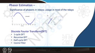
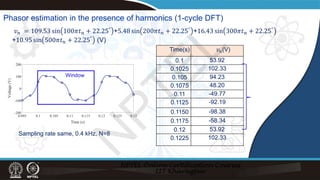
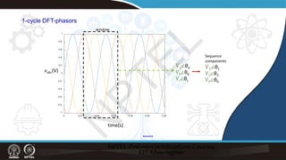
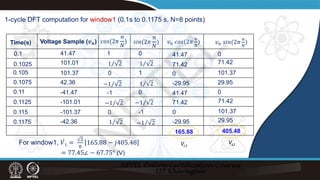
This document discusses different techniques for phasor estimation from discrete time signals, including the discrete Fourier transform (DFT). It focuses on explaining the one-cycle DFT method. The one-cycle DFT divides the signal into windows of one cycle and applies the DFT to each window to estimate the phasor. It is shown that with each new sample, the phasor estimate from the DFT advances by 45 degrees. The document also discusses applying the one-cycle DFT to signals with harmonic components and estimating sequence components from three-phase signals.

1. Power System Protection
Prof A K Pradhan
Department of Electrical Engineering
Indian Institute of Technology Kharagpur
Module 02: Phasor Estimation
Lecture 01 : Discrete Fourier Transform
N
P
T
E
L

2. Phasor estimation techniques
 Discrete Fourier Transform
 Least Square Technique
 Kalman Filter
N
P
T
E
L

3. Phasor Estimation –
Discrete Fourier Transform(DFT)
• 1-cycle DFT
• Recursive DFT
• Half-cycle DFT
• Cosine Filter
Significance of phasors in relays- usage in most of the relays
sinusoid
N
P
T
E
L

4. Discrete Fourier Transform(DFT)
Signal: 𝑣𝑣 𝑡𝑡 = 𝑉𝑉
𝑝𝑝 sin 𝜔𝜔𝑡𝑡 + 𝜃𝜃
𝑣𝑣𝑛𝑛 = 𝑉𝑉
𝑝𝑝 sin 𝜔𝜔𝑡𝑡𝑛𝑛 + 𝜃𝜃 where, 𝑡𝑡𝑛𝑛 = 𝑛𝑛∆𝑡𝑡; 𝑛𝑛 = 0,1,2, … … , ∆t =
time interval between sucessive samples
Data sampling: 8 samples/cycle
Sampling:
N
P
T
E
L

5. Phasor estimation: 1-cycle DFT
Defining
𝑉𝑉𝑟𝑟𝑟𝑟𝑟𝑟𝑟𝑟 =
2
𝑁𝑁
�
𝑛𝑛=0
𝑁𝑁−1
[𝑣𝑣𝑛𝑛 cos(2𝜋𝜋
𝑛𝑛
𝑁𝑁
)] and 𝑉𝑉𝑖𝑖𝑖𝑖𝑖𝑖𝑖𝑖 =
2
𝑁𝑁
�
𝑛𝑛=0
𝑁𝑁−1
[𝑣𝑣𝑛𝑛 sin(2𝜋𝜋
𝑛𝑛
𝑁𝑁
)]
Computed Phasor:
̇
𝑉𝑉 = 𝑉𝑉𝑟𝑟𝑟𝑟𝑟𝑟𝑟𝑟 − 𝑗𝑗𝑉𝑉𝑖𝑖𝑖𝑖𝑖𝑖𝑖𝑖 = 𝑉𝑉 ∠𝜃𝜃
Where 𝑉𝑉 = 𝑉𝑉𝑟𝑟𝑟𝑟𝑟𝑟𝑟𝑟
2
+ 𝑉𝑉𝑖𝑖𝑖𝑖𝑖𝑖𝑖𝑖
2
,𝜃𝜃 = −tan−1(
𝑉𝑉𝑖𝑖𝑖𝑖𝑖𝑖𝑖𝑖
𝑉𝑉𝑟𝑟𝑟𝑟𝑟𝑟𝑟𝑟
)
𝑣𝑣𝑛𝑛 = 𝑉𝑉
𝑝𝑝 sin 𝜔𝜔𝑡𝑡𝑛𝑛 + 𝜃𝜃
Applying 1-cycle DFT ,
Voltage phasor, ̇
𝑉𝑉 =
2
𝑁𝑁
∑𝑛𝑛=0
𝑁𝑁−1
(𝑣𝑣𝑛𝑛𝑒𝑒−𝑗𝑗
2𝜋𝜋
𝑁𝑁
𝑛𝑛
) ; 0 ≤ 𝑛𝑛 ≤ 𝑁𝑁 − 1 Where, N=number of samples in a cycle
𝑣𝑣𝑛𝑛 = 𝑛𝑛𝑡𝑡𝑡 𝑠𝑠𝑠𝑠𝑠𝑠𝑠𝑠𝑠𝑠𝑠𝑠 𝑜𝑜𝑜𝑜 𝑣𝑣(𝑡𝑡)
�
𝑛𝑛=0
𝑁𝑁−1
N
P
T
E
L

6. Data Sample window
𝑣𝑣𝑛𝑛 = 109.53 sin 100𝜋𝜋𝑡𝑡𝑛𝑛 + 22.25° (V) ,sampling rate of 0.4 kHz, N=8
Time(s)
0.1 41.47
0.1025 101.01
0.105 101.37
0.1075 42.36
0.11 -41.47
0.1125 -101.01
0.1150 -101.37
0.1175 -42.36
0.12 41.47
0.1225 101.01
Window1
Window2
𝑣𝑣𝑛𝑛(𝑉𝑉)
Window1
Window2
-Moving window
-with new sample
N
P
T
E
L

7. 1-cycle DFT computation for window1 (0.1s to 0.1175 s, N=8 points)
= 77.45∠ − 67.75° (V)
For window1,phasor ̇
𝑉𝑉 =
2
8
165.88 − 𝑗𝑗405.48
Time(s) Voltage Sample (𝒗𝒗𝒏𝒏) 𝑐𝑐𝑐𝑐𝑐𝑐(2𝜋𝜋
𝑛𝑛
𝑁𝑁
) 𝑠𝑠𝑠𝑠𝑠𝑠(2𝜋𝜋
𝑛𝑛
𝑁𝑁
) 𝑣𝑣𝑛𝑛 𝑠𝑠𝑠𝑠𝑠𝑠(2𝜋𝜋
𝑛𝑛
𝑁𝑁
)
𝑣𝑣𝑛𝑛 𝑐𝑐𝑐𝑐𝑐𝑐(2𝜋𝜋
𝑛𝑛
𝑁𝑁
)
0.1
0.1025
0.105
0.1075
0.11
0.1125
0.115
0.1175
41.47
101.01
101.37
42.36
-41.47
-101.01
-101.37
-42.36
⁄
1 2 ⁄
1 2
⁄
−1 2 ⁄
1 2
⁄
−1 2 ⁄
−1 2
⁄
1 2 ⁄
−1 2
0
0
0
0
1
1
-1
-1
41.47
41.47
71.42 71.42
-29.95 29.95
-29.95 29.95
0
0
0
0
101.37
101.37
71.42 71.42
165.88 405.48
(0 ≤ 𝑛𝑛 ≤ 𝑁𝑁 − 1)
N
P
T
E
L

8. 1-cycle DFT computation for window2 (0.1025s to 0.12 s, N=8 points)
= 77.45∠ − 22.75° (V)
For window2, ̇
𝑉𝑉 =
2
8
404.02 − 𝑗𝑗169.44
101.01
101.37
42.36
-41.47
-101.01
-101.37
-42.36
41.47
Time(s) Voltage Sample (𝒗𝒗𝒏𝒏) 𝑐𝑐𝑐𝑐𝑐𝑐(2𝜋𝜋
𝑛𝑛
𝑁𝑁
) 𝑠𝑠𝑠𝑠𝑠𝑠(2𝜋𝜋
𝑛𝑛
𝑁𝑁
) 𝑣𝑣𝑛𝑛 𝑠𝑠𝑠𝑠𝑠𝑠(2𝜋𝜋
𝑛𝑛
𝑁𝑁
)
𝑣𝑣𝑛𝑛 𝑐𝑐𝑐𝑐𝑐𝑐(2𝜋𝜋
𝑛𝑛
𝑁𝑁
)
0.1025
0.105
0.1075
0.11
0.1125
0.115
0.1175
⁄
1 2 ⁄
1 2
⁄
−1 2 ⁄
1 2
⁄
−1 2 ⁄
−1 2
⁄
1 2 ⁄
−1 2
0
0
0
0
1
1
-1
-1
0.12
101.01
101.01
71.68 71.68
29.32 -29.32
29.32 -29.32
0
0
0
0
42.36
42.36
71.68 71.68
404.02 169.44
(0 ≤ 𝑛𝑛 ≤ 𝑁𝑁 − 1)
N
P
T
E
L

9. Observations: 1-cycle DFT
With the arrival of a new sample , the window is updated and the new
phasor advances by an angle of 450 .
the magnitude of the estimated phasor is same in both windows
There is a phase difference of 450 for the estimated phasors between
window 1 and window 2 ??
 ∆t=0.02/8 corresponds to 3600/8 = 450
450 ̇
𝑉𝑉𝑊𝑊𝑊
̇
𝑉𝑉𝑊𝑊𝑊= 77.45∠ − 67.75° (V)
= 77.45∠ − 22.75° (V)
Window1
Window2
∆t
w
N
P
T
E
L

10. Phasor estimation in the presence of harmonics (1-cycle DFT)
𝑣𝑣𝑛𝑛 = 109.53 sin 100𝜋𝜋𝑡𝑡𝑛𝑛 + 22.25° +5.48 sin 200𝜋𝜋𝑡𝑡𝑛𝑛 + 22.25° +16.43 sin 300𝜋𝜋𝑡𝑡𝑛𝑛 + 22.25°
+10.95 sin 500𝜋𝜋𝑡𝑡𝑛𝑛 + 22.25° (V)
Sampling rate same, 0.4 kHz, N=8
Time(s) 𝑣𝑣𝑛𝑛(V)
0.1 53.92
0.1025 102.33
0.105 94.23
0.1075 48.20
0.11 -49.77
0.1125 -92.19
0.1150 -98.38
0.1175 -58.34
0.12 53.92
0.1225 102.33
Window
N
P
T
E
L

11. 1-cycle DFT computation for window1 (0.1s to 0.1175 s, N=8 points)
= 77.45∠ − 67.75° (V)
For window1, ̇
𝑉𝑉 =
2
8
165.91 − 𝑗𝑗405.49
53.92
102.33
94.23
48.20
-49.77
-92.19
-98.38
-58.34
Time(s) Voltage Sample (𝒗𝒗𝒏𝒏) 𝑐𝑐𝑐𝑐𝑐𝑐(2𝜋𝜋
𝑛𝑛
𝑁𝑁
) 𝑠𝑠𝑠𝑠𝑠𝑠(2𝜋𝜋
𝑛𝑛
𝑁𝑁
) 𝑣𝑣𝑛𝑛 𝑠𝑠𝑠𝑠𝑠𝑠(2𝜋𝜋
𝑛𝑛
𝑁𝑁
)
𝑣𝑣𝑛𝑛 𝑐𝑐𝑐𝑐𝑐𝑐(2𝜋𝜋
𝑛𝑛
𝑁𝑁
)
0.1
0.1025
0.105
0.1075
0.11
0.1125
0.115
0.1175
⁄
1 2 ⁄
1 2
⁄
−1 2 ⁄
1 2
⁄
−1 2 ⁄
−1 2
⁄
1 2 ⁄
−1 2
0
0
0
0
1
1
-1
-1
53.92
49.77
72.36 72.36
-34.08 34.08
-41.25 41.25
0
0
0
0
94.23
98.38
65.19 65.19
165.91 405.49
̇
𝑉𝑉𝑊𝑊𝑊= 77.45∠ − 67.75° (V)
Earlier calculation without harmonics
N
P
T
E
L

12. 1-cycle DFT-phasors
0 0.005 0.01 0.015 0.02 0.025 0.03 0.035 0.04
-1.5
-1
-0.5
0
0.5
1
1.5
time(s)
v,i v i
window
V∠θ1
I∠θ2
N
P
T
E
L

13. 1-cycle DFT-phasors
Phase information-
0 0.005 0.01 0.015 0.02 0.025 0.03 0.035 0.04
-1.5
-1
-0.5
0
0.5
1
1.5
time(s)
v,i v i
θ
V∠θ1
I∠θ2
N
P
T
E
L

14. 1-cycle DFT-phasors
0 0.01 0.02 0.03 0.04 0.05 0.06
-1
-0.8
-0.6
-0.4
-0.2
0
0.2
0.4
0.6
0.8
1
time(s)
vabc(V)
window
Va∠θa
Vb∠θb
Vc∠θc
V1∠θ1
V2∠θ2
V0∠θ0
*****
Sequence
components
N
P
T
E
L

15. Power System Protection
Prof A K Pradhan
Department of Electrical Engineering
Indian Institute of Technology Kharagpur
Module 02: Phasor Estimation
Lecture 07 : Recursive and Half Cycle DFT and Cosine Filter
N
P
T
E
L

16. Phasor estimation techniques
 Discrete Fourier Transform
Lecture 07
One cycle DFT, Recursive and Half Cycle DFT and Cosine Filter
N
P
T
E
L

17. Recursive DFT:
𝑣𝑣𝑛𝑛 = 109.53 sin 100𝜋𝜋𝑡𝑡𝑛𝑛 + 𝜃𝜃 (V), 𝑡𝑡𝑛𝑛 = 𝑛𝑛∆𝑡𝑡, where ∆𝑡𝑡=0.0025 s
1-cycle DFT for window2 (𝑣𝑣1 through 𝑣𝑣8)
̇
𝑉𝑉2 =
2
𝑁𝑁
�
𝑛𝑛=0
𝑁𝑁−1
𝑣𝑣𝑛𝑛+1𝑒𝑒−𝑗𝑗
2𝜋𝜋𝑛𝑛
𝑁𝑁
Window1 Window2
Common Portion (𝑣𝑣1 – 𝑣𝑣7)
Outgoing Sample New sample
1-cycle DFT for window1 (𝑣𝑣0 through 𝑣𝑣7)
̇
𝑉𝑉1 =
2
𝑁𝑁
�
𝑛𝑛=0
𝑁𝑁−1
𝑣𝑣𝑛𝑛𝑒𝑒−𝑗𝑗
2𝜋𝜋𝑛𝑛
𝑁𝑁
N
P
T
E
L

18. =
2
𝑁𝑁
�
𝑛𝑛=0
𝑁𝑁−2
𝑣𝑣𝑛𝑛+1𝑒𝑒−𝑗𝑗
2𝜋𝜋𝑛𝑛
𝑁𝑁 +
2
𝑁𝑁
𝑣𝑣𝑁𝑁𝑒𝑒−𝑗𝑗
2𝜋𝜋 𝑁𝑁−1
𝑁𝑁
=
2
𝑁𝑁
�
𝑛𝑛=1
𝑁𝑁−1
𝑣𝑣𝑛𝑛𝑒𝑒−𝑗𝑗
2𝜋𝜋𝑛𝑛
𝑁𝑁 𝑒𝑒𝑗𝑗
2𝜋𝜋
𝑁𝑁 +
2
𝑁𝑁
𝑣𝑣𝑁𝑁𝑒𝑒−𝑗𝑗
2𝜋𝜋 𝑁𝑁−1
𝑁𝑁
= ̇
𝑉𝑉1 −
2
𝑁𝑁
𝑣𝑣0 𝑒𝑒𝑗𝑗
2𝜋𝜋
𝑁𝑁 +
2
𝑁𝑁
𝑣𝑣𝑁𝑁𝑒𝑒−𝑗𝑗
2𝜋𝜋𝜋𝜋
𝑁𝑁 𝑒𝑒𝑗𝑗
2𝜋𝜋
𝑁𝑁
̇
𝑉𝑉2 = [ ̇
𝑉𝑉1 +
2
𝑁𝑁
(𝑣𝑣𝑁𝑁 − 𝑣𝑣0)]𝑒𝑒𝑗𝑗
2𝜋𝜋
𝑁𝑁
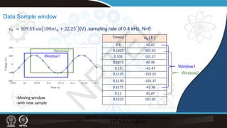
Recursive DFT:
̇
𝑉𝑉1 =
2
𝑁𝑁
�
𝑛𝑛=0
𝑁𝑁−1
𝑣𝑣𝑛𝑛𝑒𝑒−𝑗𝑗
2𝜋𝜋𝑛𝑛
𝑁𝑁
=
2
𝑁𝑁
�
𝑛𝑛=1
𝑁𝑁−1
𝑣𝑣𝑛𝑛𝑒𝑒−𝑗𝑗
2𝜋𝜋𝜋𝜋
𝑁𝑁 +
2
𝑁𝑁
𝑣𝑣0
̇
𝑉𝑉2 =
2
𝑁𝑁
�
𝑛𝑛=0
𝑁𝑁−1
𝑣𝑣𝑛𝑛+1𝑒𝑒−𝑗𝑗
2𝜋𝜋𝑛𝑛
𝑁𝑁
N
P
T
E
L

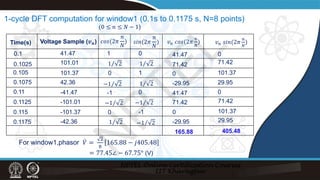
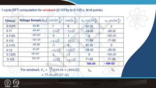
19. The phasor at the 𝑟𝑟 + 1 𝑡𝑡𝑡 instant can be written as
Earlier phasor New Sample Outgoing Sample
̇
𝑉𝑉𝑟𝑟+1 = [ ̇
𝑉𝑉
𝑟𝑟 +
2
𝑁𝑁
(𝑣𝑣N+r − 𝑣𝑣𝑟𝑟)]𝑒𝑒𝑗𝑗
2𝜋𝜋
𝑁𝑁
New phasor
Recursive DFT:
N
P
T
E
L

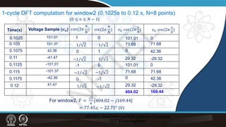
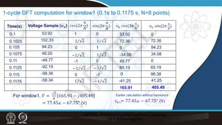
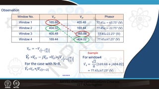
20. Recursive DFT:
Example:
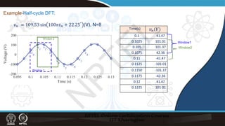
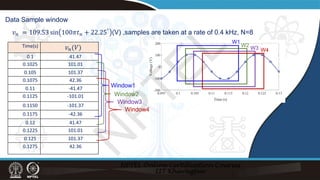
𝑣𝑣𝑛𝑛 = 109.53 sin 100𝜋𝜋𝑡𝑡𝑛𝑛 + 22.25° (V), N=8
Time(s)
0.1 41.47
0.1025 101.01
0.105 101.37
0.1075 42.36
0.11 -41.47
0.1125 -101.01
0.1150 -101.37
0.1175 -42.36
0.12 41.47
0.1225 101.01
̇
𝑉𝑉2
̇
𝑉𝑉1 = 77.45∠ − 67.75° (V)
= 77.45∠ − 22.75° (V)
̇
𝑉𝑉2 = [ ̇
𝑉𝑉1 +
2
8
(𝑣𝑣8 − 𝑣𝑣0)]𝑒𝑒𝑗𝑗
2𝜋𝜋
8
Using recursive DFT:
=[77.45∠-67.75° +
2
8
(41.47-41.47)] 𝑒𝑒𝑗𝑗
2𝜋𝜋
8
= 77.45∠ − 22.75° (V)
𝑣𝑣𝑛𝑛(𝑉𝑉)
𝑣𝑣0=
𝑣𝑣1=
𝑣𝑣2=
𝑣𝑣3=
𝑣𝑣4=
𝑣𝑣5=
𝑣𝑣6=
𝑣𝑣7=
𝑣𝑣8=
𝑣𝑣9=
N
P
T
E
L

21.  New phasor is obtained using last phasor- reducing calculation
 With larger N, this can be more advantageous
Remarks
Recursive DFT:
N
P
T
E
L

22. 𝑣𝑣𝑛𝑛 = 𝑉𝑉
𝑝𝑝 sin 𝜔𝜔𝑡𝑡𝑛𝑛 + 𝜃𝜃
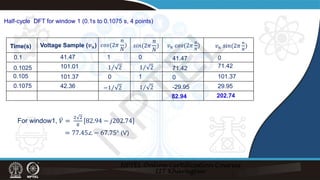
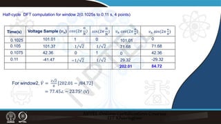
Half-cycle DFT for Phasor Calculation
1-cycle window
half-cycle window
̇
𝑉𝑉 =
2
𝑁𝑁
2
�
𝑛𝑛=0
𝑁𝑁
2
−1
𝑣𝑣𝑛𝑛𝑒𝑒−𝑗𝑗
2𝜋𝜋
𝑁𝑁
𝑛𝑛
; 0 ≤ 𝑛𝑛 ≤
𝑁𝑁
2
− 1
𝑉𝑉𝑟𝑟𝑟𝑟𝑟𝑟𝑟𝑟 =
2
𝑁𝑁
2
�
𝑛𝑛=0
𝑁𝑁
2
−1
[𝑣𝑣𝑛𝑛 cos(2𝜋𝜋
𝑛𝑛
𝑁𝑁
)]
Defining
Computed phasor: ̇
𝑉𝑉 = 𝑉𝑉𝑟𝑟𝑟𝑟𝑟𝑟𝑟𝑟 − 𝑗𝑗𝑉𝑉𝑖𝑖𝑖𝑖𝑖𝑖𝑖𝑖 = 𝑉𝑉 ∠𝜃𝜃
Where, 𝑉𝑉 = 𝑉𝑉𝑟𝑟𝑟𝑟𝑟𝑟𝑟𝑟
2
+ 𝑉𝑉𝑖𝑖𝑖𝑖𝑖𝑖𝑖𝑖
2
,𝜃𝜃 = −tan−1(
𝑉𝑉𝑖𝑖𝑖𝑖𝑖𝑖𝑖𝑖
𝑉𝑉𝑟𝑟𝑟𝑟𝑟𝑟𝑟𝑟
)
𝑉𝑉𝑖𝑖𝑖𝑖𝑖𝑖𝑖𝑖 =
2
𝑁𝑁
2
�
𝑛𝑛=0
(
𝑁𝑁
2)−1
[𝑣𝑣𝑛𝑛 sin(2𝜋𝜋
𝑛𝑛
𝑁𝑁
)]
Signal
N
P
T
E
L

23. Example-Half-cycle DFT:
𝑣𝑣𝑛𝑛 = 109.53 sin 100𝜋𝜋𝑡𝑡𝑛𝑛 + 22.25° (V), N=8
Window 1
Window 2
Time(s)
0.1 41.47
0.1025 101.01
0.105 101.37
0.1075 42.36
0.11 -41.47
0.1125 -101.01
0.1150 -101.37
0.1175 -42.36
0.12 41.47
0.1225 101.01
Window1
Window2
𝑣𝑣𝑛𝑛(𝑉𝑉)
N
P
T
E
L

24. Half-cycle DFT for window 1 (0.1s to 0.1075 s, 4 points)
For window1, ̇
𝑉𝑉 =
2 2
8
82.94 − 𝑗𝑗202.74
Time(s) Voltage Sample (𝒗𝒗𝒏𝒏) 𝑐𝑐𝑐𝑐𝑐𝑐(2𝜋𝜋
𝑛𝑛
𝑁𝑁
) 𝑠𝑠𝑠𝑠𝑠𝑠(2𝜋𝜋
𝑛𝑛
𝑁𝑁
) 𝑣𝑣𝑛𝑛 𝑠𝑠𝑠𝑠𝑠𝑠(2𝜋𝜋
𝑛𝑛
𝑁𝑁
)
𝑣𝑣𝑛𝑛 𝑐𝑐𝑐𝑐𝑐𝑐(2𝜋𝜋
𝑛𝑛
𝑁𝑁
)
0.1
0.1025
0.105
0.1075
41.47
101.01
101.37
42.36
⁄
1 2 ⁄
1 2
⁄
−1 2 ⁄
1 2
0
0
1
1
41.47
71.42 71.42
-29.95 29.95
0
0
101.37
82.94 202.74
= 77.45∠ − 67.75° (V)
N
P
T
E
L

25. Half-cycle DFT computation for window 2(0.1025s to 0.11 s, 4 points)
For window2, ̇
𝑉𝑉 =
2 2
8
202.01 − 𝑗𝑗84.72
Time(s) Voltage Sample (𝒗𝒗𝒏𝒏) 𝑐𝑐𝑐𝑐𝑐𝑐(2𝜋𝜋
𝑛𝑛
𝑁𝑁
) 𝑠𝑠𝑠𝑠𝑠𝑠(2𝜋𝜋
𝑛𝑛
𝑁𝑁
) 𝑣𝑣𝑛𝑛 𝑠𝑠𝑠𝑠𝑠𝑠(2𝜋𝜋
𝑛𝑛
𝑁𝑁
)
𝑣𝑣𝑛𝑛 𝑐𝑐𝑐𝑐𝑐𝑐(2𝜋𝜋
𝑛𝑛
𝑁𝑁
)
⁄
1 2 ⁄
1 2
⁄
−1 2 ⁄
1 2
0
0
1
1
= 77.45∠ − 22.75° (V)
0.1025
0.105
0.1075
0.11
101.01
101.37
42.36
-41.47 29.32
101.01 0
0 42.36
71.68
-29.32
71.68
202.01 84.72
N
P
T
E
L

26. Half-cycle DFT: Remarks
phasor is obtained with less number of samples.
Calculation is less as compared to one cycle DFT
During fault-it can provide phasor quickly
N
P
T
E
L

27. Cosine Filter for Phasor Calculation
̇
𝑉𝑉 =
2
𝑁𝑁
�
𝑛𝑛=0
𝑁𝑁−1
𝑣𝑣𝑛𝑛𝑒𝑒−𝑗𝑗
2𝜋𝜋
𝑁𝑁 𝑛𝑛
; 0 ≤ 𝑛𝑛 ≤ 𝑁𝑁 − 1
̇
𝑉𝑉 =𝑉𝑉
𝑐𝑐 − 𝑗𝑗𝑉𝑉
𝑠𝑠
𝑉𝑉
𝑠𝑠 =
2
𝑁𝑁
�
𝑛𝑛=0
𝑁𝑁−1
�𝑣𝑣𝑛𝑛 sin 2𝜋𝜋
𝑛𝑛
𝑁𝑁
)
R𝑒𝑒𝑒𝑒𝑒𝑒 ̇
𝑉𝑉 = 𝑉𝑉
𝑐𝑐 I𝑚𝑚𝑚𝑚𝑚𝑚 ̇
𝑉𝑉 = −𝑉𝑉
𝑠𝑠
and
𝑉𝑉
𝑐𝑐 =
2
𝑁𝑁
�
𝑛𝑛=0
𝑁𝑁−1
�𝑣𝑣𝑛𝑛 cos 2𝜋𝜋
𝑛𝑛
𝑁𝑁
)
N
P
T
E
L

28. ̇
𝑉𝑉1 = 𝑉𝑉∠𝜃𝜃
Using recursive DFT-
̇
𝑉𝑉2 = 𝑉𝑉∠(𝜃𝜃 +
2𝜋𝜋
𝑁𝑁
)
R𝑒𝑒𝑒𝑒𝑒𝑒 ̇
𝑉𝑉1 = 𝑉𝑉𝑐𝑐𝑐𝑐𝑐𝑐𝜃𝜃 = 𝑉𝑉𝑐𝑐𝑐
I𝑚𝑚𝑚𝑚𝑚𝑚 ̇
𝑉𝑉1 = 𝑉𝑉𝑠𝑠𝑠𝑠𝑠𝑠𝜃𝜃 = −𝑉𝑉𝑠𝑠𝑠
̇
𝑉𝑉3 = 𝑉𝑉∠(𝜃𝜃 +
4𝜋𝜋
𝑁𝑁
)
𝐼𝐼𝐼𝐼𝐼𝐼𝐼𝐼 ̇
𝑉𝑉𝑁𝑁
4
+1
= −𝑉𝑉
𝑠𝑠(
𝑁𝑁
4
+1)
= 𝑉𝑉 sin(𝜃𝜃 +
𝜋𝜋
2
)
𝑉𝑉
𝑠𝑠𝑠𝑠 = −𝑉𝑉
𝑐𝑐 𝑟𝑟−
𝑁𝑁
4
̇
𝑉𝑉𝑟𝑟 =𝑉𝑉
𝑐𝑐𝑟𝑟 − 𝑗𝑗𝑉𝑉
𝑠𝑠𝑠𝑠 =𝑉𝑉
𝑐𝑐𝑟𝑟+𝑗𝑗𝑉𝑉𝑐𝑐 𝑟𝑟−
𝑁𝑁
4
Let for window-1 we get,
R𝑒𝑒𝑒𝑒𝑒𝑒 ̇
𝑉𝑉 = 𝑉𝑉
𝑐𝑐 I𝑚𝑚𝑚𝑚𝑚𝑚 ̇
𝑉𝑉 = −𝑉𝑉
𝑠𝑠
and
Cosine Filter
and
̇
𝑉𝑉2 = [ ̇
𝑉𝑉1 +
2
𝑁𝑁
(𝑣𝑣𝑁𝑁 − 𝑣𝑣0)]𝑒𝑒𝑗𝑗
2𝜋𝜋
𝑁𝑁
and
= 𝑉𝑉cos 𝜃𝜃 = 𝑉𝑉𝑐𝑐𝑐
̇
𝑉𝑉𝑁𝑁
4
+1
= 𝑉𝑉∠ 𝜃𝜃 +
𝜋𝜋
2
,
̇
𝑉𝑉𝑁𝑁
4
+1
= 𝑉𝑉∠ 𝜃𝜃 +
2𝜋𝜋
𝑁𝑁
𝑁𝑁
4
,
For rth window
N
P
T
E
L

29. Data Sample window
𝑣𝑣𝑛𝑛 = 109.53 sin 100𝜋𝜋𝑡𝑡𝑛𝑛 + 22.25° (V) ,samples are taken at a rate of 0.4 kHz, N=8
Time(s)
0.1 41.47
0.1025 101.01
0.105 101.37
0.1075 42.36
0.11 -41.47
0.1125 -101.01
0.1150 -101.37
0.1175 -42.36
0.12 41.47
0.1225 101.01
0.125 101.37
0.1275 42.36
Window1
Window2
𝑣𝑣𝑛𝑛(𝑉𝑉)
W1
W2
Window3
Window4
W3 W4
N
P
T
E
L

30. 1-cycle DFT computation for window1 (0.1s to 0.1175 s, N=8 points)
= 77.45∠ − 67.75° (V)
For window1, ̇
𝑉𝑉1 =
2
8
165.88 − 𝑗𝑗405.48
Time(s) Voltage Sample (𝒗𝒗𝒏𝒏) 𝑐𝑐𝑐𝑐𝑐𝑐(2𝜋𝜋
𝑛𝑛
𝑁𝑁
) 𝑠𝑠𝑠𝑠𝑠𝑠(2𝜋𝜋
𝑛𝑛
𝑁𝑁
) 𝑣𝑣𝑛𝑛 𝑠𝑠𝑠𝑠𝑠𝑠(2𝜋𝜋
𝑛𝑛
𝑁𝑁
)
𝑣𝑣𝑛𝑛 𝑐𝑐𝑐𝑐𝑐𝑐(2𝜋𝜋
𝑛𝑛
𝑁𝑁
)
0.1
0.1025
0.105
0.1075
0.11
0.1125
0.115
0.1175
41.47
101.01
101.37
42.36
-41.47
-101.01
-101.37
-42.36
⁄
1 2 ⁄
1 2
⁄
−1 2 ⁄
1 2
⁄
−1 2 ⁄
−1 2
⁄
1 2 ⁄
−1 2
0
0
0
0
1
1
-1
-1
41.47
41.47
71.42 71.42
-29.95 29.95
-29.95 29.95
0
0
0
0
101.37
101.37
71.42 71.42
165.88 405.48
Vc1
Vs1
N
P
T
E
L

31. 1-cycle DFT computation for window2 (0.1025s to 0.12 s, N=8 points)
= 77.45∠ − 22.75° (V)
For window2, ̇
𝑉𝑉2 =
2
8
404.02 − 𝑗𝑗169.44
101.01
101.37
42.36
-41.47
-101.01
-101.37
-42.36
41.47
Time(s) Voltage Sample (𝒗𝒗𝒏𝒏) 𝑐𝑐𝑐𝑐𝑐𝑐(2𝜋𝜋
𝑛𝑛
𝑁𝑁
) 𝑠𝑠𝑠𝑠𝑠𝑠(2𝜋𝜋
𝑛𝑛
𝑁𝑁
) 𝑣𝑣𝑛𝑛 𝑠𝑠𝑠𝑠𝑠𝑠(2𝜋𝜋
𝑛𝑛
𝑁𝑁
)
𝑣𝑣𝑛𝑛 𝑐𝑐𝑐𝑐𝑐𝑐(2𝜋𝜋
𝑛𝑛
𝑁𝑁
)
0.1025
0.105
0.1075
0.11
0.1125
0.115
0.1175
⁄
1 2 ⁄
1 2
⁄
−1 2 ⁄
1 2
⁄
−1 2 ⁄
−1 2
⁄
1 2 ⁄
−1 2
0
0
0
0
1
1
-1
-1
0.12
101.01
101.01
71.68 71.68
29.32 -29.32
29.32 -29.32
0
0
0
0
42.36
42.36
71.68 71.68
404.02 169.44
Vc2
Vs2
N
P
T
E
L

32. 1-cycle DFT computation for window3 (0.105s to 0.1225 s, N=8 points)
= 77.45∠22.25° (V)
For window3, ̇
𝑉𝑉3 =
2
8
405.48 + 𝑗𝑗165.88
101.37 101.37 0
42.36 29.95 29.95
-41.47 0 -41.47
-101.01 71.42 -71.42
-101.37 101.37 0
-42.36 29.95 29.95
41.47 0 -41.47
101.01 71.42 -71.42
Time(s) Voltage Sample (𝒗𝒗𝒏𝒏) 𝑐𝑐𝑐𝑐𝑐𝑐(2𝜋𝜋
𝑛𝑛
𝑁𝑁
) 𝑠𝑠𝑠𝑠𝑠𝑠(2𝜋𝜋
𝑛𝑛
𝑁𝑁
) 𝑣𝑣𝑛𝑛 𝑠𝑠𝑠𝑠𝑠𝑠(2𝜋𝜋
𝑛𝑛
𝑁𝑁
)
𝑣𝑣𝑛𝑛 𝑐𝑐𝑐𝑐𝑐𝑐(2𝜋𝜋
𝑛𝑛
𝑁𝑁
)
0.105
0.1075
0.11
0.1125
0.115
0.1175
⁄
1 2 ⁄
1 2
⁄
−1 2 ⁄
1 2
⁄
−1 2 ⁄
−1 2
⁄
1 2 ⁄
−1 2
0
0
0
0
1
1
-1
-1
0.12
405.48 -165.88
0.1225
Vc3
Vs3
N
P
T
E
L

33. 1-cycle DFT computation for window4 (0.1075s to 0.125 s, N=8 points)
= 77.45∠67.25° (V)
For window4, ̇
𝑉𝑉4 =
2
8
169.44 + 𝑗𝑗404.02
42.36 42.36 0
-41.47 -29.32 -29.32
-101.01 0 -101.01
-101.37 71.68 -71.68
-42.36 42.36 0
41.47 -29.32 -29.32
101.01 0 -101.01
101.37 71.68 -71.68
Time(s) Voltage Sample (𝒗𝒗𝒏𝒏) 𝑐𝑐𝑐𝑐𝑐𝑐(2𝜋𝜋
𝑛𝑛
𝑁𝑁
) 𝑠𝑠𝑠𝑠𝑠𝑠(2𝜋𝜋
𝑛𝑛
𝑁𝑁
) 𝑣𝑣𝑛𝑛 𝑠𝑠𝑠𝑠𝑠𝑠(2𝜋𝜋
𝑛𝑛
𝑁𝑁
)
𝑣𝑣𝑛𝑛 𝑐𝑐𝑐𝑐𝑐𝑐(2𝜋𝜋
𝑛𝑛
𝑁𝑁
)
⁄
1 2 ⁄
1 2
⁄
−1 2 ⁄
1 2
⁄
−1 2 ⁄
−1 2
⁄
1 2 ⁄
−1 2
0
0
0
0
1
1
-1
-1
169.44 - 404.02
0.1075
0.11
0.1125
0.115
0.1175
0.12
0.125
0.1225
Vc4
Vs4
N
P
T
E
L

34. Observation
Window No. Vcr Vsr Phasor
Window 1 165.88 405.48
Window 2 404.02 169.44
Window 3 405.48 -165.88
Window 4 169.44 -404.02
77.45∠ − 67.75° (V)
77.45∠ − 22.75° (V)
77.45∠22.25° (V)
77.45∠67.25° (V)
𝑉𝑉
𝑠𝑠𝑠𝑠 = −𝑉𝑉
𝑐𝑐 𝑟𝑟−
𝑁𝑁
4
̇
𝑉𝑉
𝑟𝑟 =𝑉𝑉
𝑐𝑐𝑟𝑟 − 𝑗𝑗𝑉𝑉
𝑠𝑠𝑠𝑠 =𝑉𝑉
𝑐𝑐𝑟𝑟+𝑗𝑗𝑉𝑉𝑐𝑐 𝑟𝑟−
𝑁𝑁
4
For the case with N=8,
̇
𝑉𝑉𝑟𝑟=𝑉𝑉
𝑐𝑐𝑐𝑐+𝑗𝑗𝑗𝑗𝑐𝑐 𝑟𝑟−2
Example
For window4
̇
𝑉𝑉4 =
2
8
169.44 + 𝑗𝑗404.02
= 77.45∠67.25° (V)
*****
N
P
T
E
L

35. Power System Protection
Prof A K Pradhan
Department of Electrical Engineering
Indian Institute of Technology Kharagpur
Module 02: Phasor Estimation
Lecture 08 : Least Square Technique
N
P
T
E
L

36. Phasor estimation techniques
• Least Square Estimation technique
• Application to Phasor estimation
Lecture 08 Least Square Technique
N
P
T
E
L

37. Least Square Estimation
Consider a set of measurements that satisfies
𝑎𝑎 + 𝑏𝑏𝑡𝑡0 = 𝑚𝑚0
𝑎𝑎 + 𝑏𝑏𝑡𝑡𝑛𝑛−1 = 𝑚𝑚𝑛𝑛−1
𝑎𝑎 + 𝑏𝑏𝑏𝑏 = 𝑚𝑚
m is the measurement set, ‘t’ the associated time index
a and b are unknown system parameters to be obtained
.
.
Where,
For ‘a set of n’ number of measurements, taken at a regular interval
.
.
.
.
𝑤𝑤𝑤𝑤𝑤𝑤𝑤𝑤𝑤 𝑚𝑚0, 𝑚𝑚1 … . 𝑚𝑚𝑛𝑛−1 are the measurements and 𝑡𝑡0, 𝑡𝑡1 … . 𝑡𝑡𝑛𝑛−1 are corresponding time index
𝑎𝑎 + 𝑏𝑏𝑡𝑡1 = 𝑚𝑚1
N
P
T
E
L

38. If �
𝑎𝑎 and �
𝑏𝑏 are the estimated values
�
𝑎𝑎 + �
𝑏𝑏𝑡𝑡0 − 𝑚𝑚0 = 𝜖𝜖1
�
𝑎𝑎 + �
𝑏𝑏𝑡𝑡1 − 𝑚𝑚1 = 𝜖𝜖2
�
𝑎𝑎 + �
𝑏𝑏𝑡𝑡𝑛𝑛−1 − 𝑚𝑚𝑛𝑛−1 = 𝜖𝜖𝑛𝑛−1
for 𝑚𝑚0, 𝑚𝑚2 … . 𝑚𝑚𝑛𝑛−1 are the measurements.
𝜖𝜖0, 𝜖𝜖2 … . 𝜖𝜖𝑛𝑛−1 are the errors (residues)
Where,
Least Square Estimation
1 𝑡𝑡0
1 𝑡𝑡1
. .
. .
1 𝑡𝑡𝑛𝑛−1
�
𝑎𝑎
�
𝑏𝑏
−
𝑚𝑚0
𝑚𝑚1
.
.
𝑚𝑚𝑛𝑛−1
=
𝜖𝜖0
𝜖𝜖1
.
.
𝜖𝜖𝑛𝑛−1
[A] [X] – [m] = [𝜖𝜖]
unknown
[𝜖𝜖]= [A][X] – [m]
n ×1
2 ×1
n ×2
n ×1
measurement
.
.
.
.
N
P
T
E
L

39. Least Square Estimation
[𝜖𝜖]= [A][X] – [m]
𝜖𝜖 𝑇𝑇 𝜖𝜖 = 𝐴𝐴𝑋𝑋 − 𝑚𝑚 𝑇𝑇 𝐴𝐴𝑋𝑋 − 𝑚𝑚
= [ 𝐴𝐴𝑋𝑋 𝑇𝑇
− 𝑚𝑚 𝑇𝑇
] [𝐴𝐴𝑋𝑋 − 𝑚𝑚]
= 𝐴𝐴𝑋𝑋 𝑇𝑇 𝐴𝐴𝐴𝐴 + 𝑚𝑚 𝑇𝑇[𝑚𝑚] − 𝐴𝐴𝑋𝑋 𝑇𝑇 𝑚𝑚 − 𝑚𝑚 𝑇𝑇 𝐴𝐴𝐴𝐴
𝑚𝑚 𝑇𝑇 𝐴𝐴𝐴𝐴 = 𝑚𝑚𝑇𝑇𝐴𝐴𝐴𝐴 𝑇𝑇
𝑚𝑚 : n ×1 𝑚𝑚 𝑇𝑇
: 1 × n
[A]: n × 2
[X]: 2 × 1
𝐴𝐴𝐴𝐴 : n × 1
𝑚𝑚 𝑇𝑇
𝐴𝐴𝐴𝐴 : 1 × 1
For the 1 × 1 matrix,
= 𝐴𝐴𝑋𝑋 𝑇𝑇[𝑚𝑚]
= [𝑋𝑋]𝑇𝑇
[𝐴𝐴]𝑇𝑇
[𝑚𝑚]
𝜖𝜖 𝑇𝑇[𝜖𝜖] = 𝑋𝑋𝑇𝑇𝐴𝐴𝑇𝑇[𝐴𝐴𝑋𝑋] + 𝑚𝑚𝑇𝑇 𝑚𝑚 − 2 𝑋𝑋 𝑇𝑇 𝐴𝐴 𝑇𝑇[𝑚𝑚]
Here
N
P
T
E
L

40. Least Square Estimation
Differentiating the above equation w.r.t. [𝑋𝑋]
2[𝐴𝐴]𝑇𝑇
𝐴𝐴 [X] − 2 𝐴𝐴 𝑇𝑇
[𝑚𝑚] = 0
[𝐴𝐴]𝑇𝑇
𝐴𝐴 [𝑋𝑋] = 𝐴𝐴 𝑇𝑇
[𝑚𝑚]
𝑋𝑋 = 𝐴𝐴𝑇𝑇
𝐴𝐴 −1
[𝐴𝐴]𝑇𝑇
[𝑚𝑚]
𝜖𝜖 𝑇𝑇[𝜖𝜖] = 𝑋𝑋 𝑇𝑇 𝐴𝐴 𝑇𝑇[𝐴𝐴𝑋𝑋] + 𝑚𝑚𝑇𝑇 𝑚𝑚 − 2 𝑋𝑋 𝑇𝑇 𝐴𝐴 𝑇𝑇[𝑚𝑚]
unknown
when[𝐴𝐴] is a square matrix, the pseudo inverse becomes invese of [A]
𝑓𝑓𝑓𝑓𝑓𝑓 𝑡𝑡𝑡𝑡𝑡 𝑠𝑠𝑠𝑠𝑠𝑠𝑠𝑠𝑠𝑠𝑠𝑠 𝑎𝑎 + 𝑏𝑏𝑏𝑏 = 𝑚𝑚
N
P
T
E
L

41. Least Square Estimation for Phasor estimation
where 𝑣𝑣𝑛𝑛 voltage sample at 𝑡𝑡𝑛𝑛 , 𝑉𝑉, 𝜃𝜃 are to be found out
𝑣𝑣𝑛𝑛 = 𝑉𝑉 sin 𝜔𝜔𝑡𝑡𝑛𝑛 + 𝜃𝜃
𝑣𝑣1 = 𝑉𝑉 𝑠𝑠𝑠𝑠𝑠𝑠 𝜔𝜔𝑡𝑡1 + 𝜃𝜃
= 𝑉𝑉 𝑠𝑠𝑠𝑠𝑠𝑠 𝜔𝜔𝑡𝑡1 𝑐𝑐𝑐𝑐𝑐𝑐 𝜃𝜃 + 𝑉𝑉 sin 𝜃𝜃 cos 𝜔𝜔𝑡𝑡1
at 𝑡𝑡 = 𝑡𝑡1,
= 𝑉𝑉 cos 𝜃𝜃sin 𝜔𝜔𝑡𝑡1 + 𝑉𝑉 sin 𝜃𝜃 cos 𝜔𝜔𝑡𝑡1
= 𝑎𝑎11 𝑋𝑋1 + 𝑎𝑎12𝑋𝑋2 𝑤𝑤𝑤𝑤𝑤𝑤𝑤 𝑎𝑎11 = sin 𝜔𝜔𝑡𝑡1 , 𝑎𝑎12 = cos(𝜔𝜔𝑡𝑡1)
at 𝑡𝑡 = 𝑡𝑡0,
= 𝑉𝑉 cos 𝜃𝜃sin 𝜔𝜔𝑡𝑡0 + 𝑉𝑉 sin 𝜃𝜃 cos 𝜔𝜔𝑡𝑡0
𝑣𝑣0 = 𝑉𝑉 𝑠𝑠𝑠𝑠𝑠𝑠 𝜔𝜔𝑡𝑡0 + 𝜃𝜃
= 𝑉𝑉 𝑠𝑠𝑠𝑠𝑠𝑠 𝜔𝜔𝑡𝑡0 𝑐𝑐𝑐𝑐𝑐𝑐 𝜃𝜃 + 𝑉𝑉 sin 𝜃𝜃 cos 𝜔𝜔𝑡𝑡0
two unknowns?
= 𝑎𝑎01𝑋𝑋1 + 𝑎𝑎02𝑋𝑋2
𝑋𝑋1 = 𝑉𝑉 𝑐𝑐𝑐𝑐𝑐𝑐 𝜃𝜃, 𝑋𝑋2 = 𝑉𝑉 𝑠𝑠𝑠𝑠𝑠𝑠 𝜃𝜃
𝑎𝑎01 = sin 𝜔𝜔𝑡𝑡0 , 𝑎𝑎02 = cos(𝜔𝜔𝑡𝑡0)
Where,
N
P
T
E
L

42. Least Square Estimation for Phasor
𝑎𝑎01𝑋𝑋1 + 𝑎𝑎02𝑋𝑋2 = 𝑣𝑣0
𝑎𝑎11𝑋𝑋1 + 𝑎𝑎12𝑋𝑋2 = 𝑣𝑣1
.
.
𝑎𝑎(𝑛𝑛−1)1𝑋𝑋1 + 𝑎𝑎(𝑛𝑛−1)2𝑋𝑋2 = 𝑣𝑣𝑛𝑛−1
[𝐴𝐴] =
𝑎𝑎01 𝑎𝑎02
𝑎𝑎11 𝑎𝑎12
. .
. .
𝑎𝑎(𝑛𝑛−1)1 𝑎𝑎(𝑛𝑛−1)2
[𝑋𝑋] =
𝑋𝑋1
𝑋𝑋2 [𝑚𝑚] =
𝑣𝑣0
𝑣𝑣1
.
.
𝑣𝑣𝑛𝑛−1
𝑎𝑎01 = sin(𝜔𝜔𝑡𝑡0) 𝑎𝑎02 = cos(𝜔𝜔𝑡𝑡0)
𝑎𝑎11 = sin(𝜔𝜔𝑡𝑡1) 𝑎𝑎12 = cos(𝜔𝜔𝑡𝑡1)
𝑎𝑎(n−1)1 = sin(𝜔𝜔𝑡𝑡(n−1)) 𝑎𝑎 n−1 2 = cos(𝜔𝜔𝑡𝑡(n−1))
.
.
.
.
.
.
𝑤𝑤𝑤𝑤𝑤𝑤𝑤𝑤𝑤
𝑤𝑤𝑤𝑤𝑤𝑤𝑤𝑤𝑤
unknowns
measurements
N
P
T
E
L

43. 𝑋𝑋1 = 𝑉𝑉 𝑐𝑐𝑐𝑐𝑐𝑐 𝜃𝜃 𝑋𝑋2 = 𝑉𝑉 𝑠𝑠𝑠𝑠𝑠𝑠 𝜃𝜃
𝑉𝑉 = 𝑋𝑋1
2
+ 𝑋𝑋2
2
Vrms =
𝑉𝑉
2
Number of unknowns = 2, we need at least 2 samples to obtain the phasor
or more can be included.
Say, with 1 cycle data in the window, for 50 Hz and sampling rate 0.4 kHz, 8 samples
Size of X = 2 x 1
Size of A = 8 x 2
Size of m = 8 x 1
𝜃𝜃 = tan−1
𝑋𝑋2
𝑋𝑋1
Least Square Estimation for Phasor
𝐴𝐴 𝑋𝑋 = [𝑚𝑚]
𝑋𝑋 = 𝐴𝐴𝑇𝑇𝐴𝐴 −1[𝐴𝐴]𝑇𝑇 [𝑚𝑚]
N
P
T
E
L

44. samples are taken at a rate of 0.4 kHz,
V 𝑡𝑡 = 109.53 sin 100𝜋𝜋𝜋𝜋 + 22.25°
(V) , ∆𝑡𝑡 = 0.0025 𝑠𝑠
Least Square Estimation for Phasor
Example1
Time(s)
0.1 41.47
0.1025 101.01
0.105 101.37
0.1075 42.36
0.11 -41.47
0.1125 -101.01
0.1150 -101.37
0.1175 -42.36
0.12 41.47
0.1225 101.01
𝑣𝑣𝑛𝑛(𝑉𝑉)
N
P
T
E
L

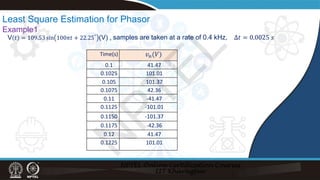
45. Time(s)
0.1 41.47
0.1025 101.01
0.105 101.37
0.1075 42.36
0.11 -41.47
0.1125 -101.01
0.1150 -101.37
0.1175 -42.36
0.12 41.47
0.1225 101.01
𝑣𝑣𝑛𝑛(𝑉𝑉)
t0
t1
Least Square Estimation for Phasor
Example1..
[𝑚𝑚] =
41.47
101.01
[𝑋𝑋] =
𝑉𝑉 cos 𝜃𝜃
𝑉𝑉 sin 𝜃𝜃
𝜔𝜔 = 2𝜋𝜋𝜋𝜋 = 2𝜋𝜋 50 = 100𝜋𝜋
[𝐴𝐴] =
sin 𝜔𝜔𝑡𝑡0 cos 𝜔𝜔𝑡𝑡0
sin 𝜔𝜔𝑡𝑡1 cos 𝜔𝜔𝑡𝑡1
=
0 1
1
2
1
2
assigning time for the calculation window, t0 = 0.0 s and t1 = 0.0025s
in [A]
For the corresponding samples as marked in the table
𝑋𝑋 = 𝐴𝐴𝑇𝑇𝐴𝐴 −1[𝐴𝐴]𝑇𝑇 [𝑚𝑚]
N
P
T
E
L

46. [𝐴𝐴]𝑇𝑇[𝐴𝐴] =
0
1
2
1
1
2
0 1
1
2
1
2
=
0.5 0.5
0.5 1.5
[ 𝐴𝐴𝑇𝑇𝐴𝐴 ]−1=
3 −1
−1 1
𝐴𝐴𝑇𝑇𝐴𝐴 −1[𝐴𝐴]𝑇𝑇=
3 −1
−1 1
0
1
2
1
1
2
=
−1 1.4142
1 0
𝑋𝑋 =
−1 1.4142
1 0
41.47
101.01
=
101.37
41.47
Least Square Estimation for Phasor
Example1…
𝑋𝑋 = 𝐴𝐴𝑇𝑇𝐴𝐴 −1[𝐴𝐴]𝑇𝑇 [𝑚𝑚]
N
P
T
E
L

47. 𝑉𝑉 = 𝑋𝑋1
2
+ 𝑋𝑋2
2 = 109 ⋅ 53 𝑉𝑉 , 𝑉𝑉(𝑟𝑟𝑟𝑟𝑟𝑟) = 77.45 (V)
𝜃𝜃 = tan−1
𝑋𝑋2
𝑋𝑋1
= 22.250
Estimated phasor is 77.45∠22.25° (V)
Least Square Estimation for Phasor
Example1..
N
P
T
E
L

48. Time(s)
0.1 41.47
0.1025 101.01
0.105 101.37
0.1075 42.36
0.11 -41.47
0.1125 -101.01
0.1150 -101.37
0.1175 -42.36
0.12 41.47
0.1225 101.01
𝑣𝑣𝑛𝑛(𝑉𝑉)
t0
t1
[𝑚𝑚] =
101.01
101.37
[𝑋𝑋] =
𝑉𝑉 cos 𝜃𝜃
𝑉𝑉 sin 𝜃𝜃
𝜔𝜔 = 2𝜋𝜋𝜋𝜋 = 2𝜋𝜋 50 = 100𝜋𝜋
[𝐴𝐴] =
sin 𝜔𝜔𝑡𝑡0 cos 𝜔𝜔𝑡𝑡0
sin 𝜔𝜔𝑡𝑡1 cos 𝜔𝜔𝑡𝑡1
=
0 1
1
2
1
2
with t0 = 0.0 s and t1 = 0.0025s for matrix A
For the corresponding samples as marked in the table
Least Square Estimation for Phasor
Example2- Different window
𝑋𝑋 = 𝐴𝐴𝑇𝑇𝐴𝐴 −1[𝐴𝐴]𝑇𝑇 [𝑚𝑚]
N
P
T
E
L

49. [𝐴𝐴]𝑇𝑇
[𝐴𝐴] =
0
1
2
1
1
2
0 1
1
2
1
2
=
0.5 0.5
0.5 1.5
𝐴𝐴𝑇𝑇𝐴𝐴 −1 =
3 −1
−1 1
𝐴𝐴𝑇𝑇𝐴𝐴 −1[𝐴𝐴]𝑇𝑇=
3 −1
−1 1
0
1
2
1
1
2
=
−1 1.4142
1 0
𝑋𝑋 =
−1 1.4142
1 0
101.01
101.37
=
42.36
101.01
Least Square Estimation for Phasor
Example2..
𝑋𝑋 = 𝐴𝐴𝑇𝑇𝐴𝐴 −1[𝐴𝐴]𝑇𝑇 [𝑚𝑚]
N
P
T
E
L

50. 𝑉𝑉 = 𝑋𝑋1
2
+ 𝑋𝑋2
2 = 109 ⋅ 53 (V)
𝑉𝑉(𝑟𝑟𝑟𝑟𝑟𝑟) = 77.45 (V)
𝜃𝜃 = tan−1
𝑋𝑋2
𝑋𝑋1
= 67.250
Estimated phasor is 77.45∠67.25° (V)
Least Square Estimation for Phasor
Example2..
in the second window we got 77.45∠67.25° (V).
There is a phase shift of 45°which is correct
for the 0.4 kHz sampling for 50 Hz signal N=8
In first window, we got phasor 77.45∠22.25° (V)
N
P
T
E
L

51. Phasor estimation in the presence of harmonics (Least Square Estimation)
𝑣𝑣𝑛𝑛 = 109.53 sin 100𝜋𝜋𝑡𝑡𝑛𝑛 + 22.25° +5.48 sin 200𝜋𝜋𝑡𝑡𝑛𝑛 + 22.25° +16.43 sin 300𝜋𝜋𝑡𝑡𝑛𝑛 + 22.25°
+10.95 sin 500𝜋𝜋𝑡𝑡𝑛𝑛 + 22.25° (V)
Sampling rate same, 0.4 kHz,50 Hz, N=8
Time(s) 𝑣𝑣𝑛𝑛(V)
0.1 53.92
0.1025 102.33
0.105 94.23
0.1075 48.20
0.11 -49.77
0.1125 -92.19
0.1150 -98.38
0.1175 -58.34
0.12 53.92
0.1225 102.33
Example 3
N
P
T
E
L

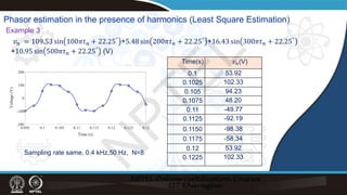
52. Time(s) 𝑣𝑣𝑛𝑛(V)
0.1 53.92
0.1025 102.33
0.105 94.23
0.1075 48.20
0.11 -49.77
0.1125 -92.19
0.1150 -98.38
0.1175 -58.34
0.12 53.92
0.1225 102.33
t0
t1 [𝑚𝑚] =
53.92
102.33
[𝑋𝑋] =
𝑉𝑉 cos 𝜃𝜃
𝑉𝑉 sin 𝜃𝜃
𝜔𝜔 = 2𝜋𝜋𝜋𝜋 = 2𝜋𝜋 50 = 100𝜋𝜋
[𝐴𝐴] =
sin 𝜔𝜔𝑡𝑡0 cos 𝜔𝜔𝑡𝑡0
sin 𝜔𝜔𝑡𝑡1 cos 𝜔𝜔𝑡𝑡1
=
0 1
1
2
1
2
Only with 2 measurements:
Example 3:
𝑋𝑋 = 𝐴𝐴𝑇𝑇𝐴𝐴 −1[𝐴𝐴]𝑇𝑇 [𝑚𝑚]
N
P
T
E
L

53. [𝐴𝐴]𝑇𝑇
[𝐴𝐴] =
0
1
2
1
1
2
0 1
1
2
1
2
=
0.5 0.5
0.5 1.5
𝐴𝐴𝑇𝑇𝐴𝐴 −1 =
3 −1
−1 1
𝐴𝐴𝑇𝑇𝐴𝐴 −1[𝐴𝐴]𝑇𝑇=
3 −1
−1 1
0
1
2
1
1
2
=
−1 1.4142
1 0
[𝑋𝑋] =
−1 1.4142
1 0
53.92
102.33
=
90.80
53.91
Example 3..
N
P
T
E
L

54. 𝑉𝑉 = 𝑋𝑋1
2
+ 𝑋𝑋2
2 = 105.6 (𝑉𝑉), 𝑉𝑉(𝑟𝑟𝑟𝑟𝑟𝑟) = 74.67 (V)
𝜃𝜃 = tan−1
𝑋𝑋2
𝑋𝑋1
= 30.70
Estimated phasor is 74.67∠30.7° (V)
correct phasor 77.45∠22.25° (V)
Example 3..
N
P
T
E
L

55. Time(s) 𝑣𝑣𝑛𝑛(V)
0.1 53.92
0.1025 102.33
0.105 94.23
0.1075 48.20
0.11 -49.77
0.1125 -92.19
0.1150 -98.38
0.1175 -58.34
0.12 53.92
0.1225 102.33
[𝑚𝑚] =
53.92
102.33
94.23
48.20
−49.77
−92.19
−98.38
−58.34
[𝑋𝑋] =
𝑉𝑉 cos 𝜃𝜃
𝑉𝑉 sin 𝜃𝜃
𝜔𝜔 = 2𝜋𝜋𝜋𝜋 = 2𝜋𝜋 50 = 100𝜋𝜋
With 8 measurements (1-cycle window)
t0
t1
t2
t3
t4
t5
t6
t7
[𝐴𝐴] =
sin 𝜔𝜔𝑡𝑡0 cos 𝜔𝜔𝑡𝑡0
sin 𝜔𝜔𝑡𝑡1 cos 𝜔𝜔𝑡𝑡1
sin 𝜔𝜔𝑡𝑡2
sin 𝜔𝜔𝑡𝑡3
sin 𝜔𝜔𝑡𝑡4
sin 𝜔𝜔𝑡𝑡5
sin 𝜔𝜔𝑡𝑡6
sin 𝜔𝜔𝑡𝑡7
cos 𝜔𝜔𝑡𝑡2
cos 𝜔𝜔𝑡𝑡3
cos 𝜔𝜔𝑡𝑡4
cos 𝜔𝜔𝑡𝑡5
cos 𝜔𝜔𝑡𝑡6
cos 𝜔𝜔𝑡𝑡7
=
0 1
1
2
1
2
1
1
2
0
−
1
2
−1
−
1
2
−
0
1
2
−1
−
1
2
0
1
2
with t0 = 0.0 s and t1 = 0.0025s … t7 =0.175 s
for matrix A
Example 3:
N
P
T
E
L

56. 𝐴𝐴𝑇𝑇
𝐴𝐴 −1
𝐴𝐴𝑇𝑇
=
=
101.37
41.47
0 0.1768 0.25 0.1768 0 −0.1768 −0.25 −0.1768
0.25 0.1768 0 −0.1768 −0.25 −0.1768 0 0.1768
𝑉𝑉 = 𝑋𝑋1
2
+ 𝑋𝑋2
2 = 109 ⋅ 53 (𝑉𝑉) 𝑉𝑉(𝑟𝑟𝑟𝑟𝑟𝑟) = 77.45 (V)
𝜃𝜃 = tan−1
𝑋𝑋2
𝑋𝑋1
= 22.250
Estimated phasor is 77.45∠22.25° (V)
This is correct the phasor.
𝑋𝑋 = 𝐴𝐴𝑇𝑇
𝐴𝐴 −1
[𝐴𝐴]𝑇𝑇
[𝑚𝑚]
N
P
T
E
L

57. Estimation of harmonic component (using Least Square Estimation)
𝑣𝑣𝑛𝑛 = 𝑉𝑉1 sin 𝜔𝜔𝑡𝑡𝑛𝑛 + 𝜃𝜃1 +𝑉𝑉2 sin 2𝜔𝜔𝑡𝑡𝑛𝑛 + 𝜃𝜃2
𝑣𝑣𝑛𝑛 = 𝑉𝑉1 𝑠𝑠𝑠𝑠𝑠𝑠 𝜔𝜔𝑡𝑡n 𝑐𝑐𝑐𝑐𝑐𝑐 𝜃𝜃1 + 𝑉𝑉1 sin 𝜃𝜃1 cos 𝜔𝜔𝑡𝑡n +𝑉𝑉2 𝑠𝑠𝑠𝑠𝑠𝑠 2𝜔𝜔𝑡𝑡n 𝑐𝑐𝑐𝑐𝑐𝑐 𝜃𝜃2 + 𝑉𝑉2 sin 𝜃𝜃2 cos 2𝜔𝜔𝑡𝑡n
Say we need 2nd harmonic component to be estimated with fundamental
A =
sin 𝜔𝜔𝑡𝑡0 cos 𝜔𝜔𝑡𝑡0 sin 2𝜔𝜔𝑡𝑡0 cos 2𝜔𝜔𝑡𝑡0
sin 𝜔𝜔𝑡𝑡1 cos 𝜔𝜔𝑡𝑡1 sin 2𝜔𝜔𝑡𝑡1 cos 2𝜔𝜔𝑡𝑡1
⋮ ⋮ ⋮ ⋮
⋮ ⋮ ⋮ ⋮
sin 𝜔𝜔𝑡𝑡n−1 cos 𝜔𝜔𝑡𝑡n−1 sin 2𝜔𝜔𝑡𝑡n−1 cos 2𝜔𝜔𝑡𝑡n−1
𝑚𝑚 =
𝑣𝑣0
𝑣𝑣1
⋮
⋮
𝑣𝑣n
𝑉𝑉1 = 𝑋𝑋1
2
+ 𝑋𝑋2
2 V1rms =
𝑉𝑉1
2
𝜃𝜃1 = tan−1
𝑋𝑋2
𝑋𝑋1
𝑋𝑋 =
𝑉𝑉1 𝑐𝑐𝑐𝑐𝑐𝑐 𝜃𝜃1
𝑉𝑉1 𝑠𝑠𝑠𝑠𝑠𝑠 𝜃𝜃1
𝑉𝑉2 𝑐𝑐𝑐𝑐𝑐𝑐 𝜃𝜃2
𝑉𝑉2 𝑠𝑠𝑠𝑠𝑠𝑠 𝜃𝜃2
𝑉𝑉2 = 𝑋𝑋3
2
+ 𝑋𝑋4
2 𝜃𝜃2 = tan−1
𝑋𝑋4
𝑋𝑋3
V2rms =
𝑉𝑉2
2
𝑋𝑋2
𝑋𝑋1
𝑋𝑋3
𝑋𝑋4
2nd harmonic
𝑋𝑋 = 𝐴𝐴𝑇𝑇𝐴𝐴 −1[𝐴𝐴]𝑇𝑇 [𝑚𝑚]
N
P
T
E
L

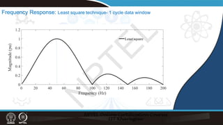
58. Remarks
Least square estimation- provides phasors like DFT
It can manage with less number of samples for pure sinusoid
But with harmonics– it is able to filter out with 1-cycle of data
—similar to 1-cycle DFT
- We can incorporate harmonics also and get the magnitude and phase.
To reduce computation- matrix- [A] is fixed for a given window size and
signal sampling rate—so also the 𝐴𝐴𝑇𝑇𝐴𝐴 −1[𝐴𝐴]𝑇𝑇
∗∗∗∗∗
N
P
T
E
L

59. Power System Protection
Prof A K Pradhan
Electrical Engineering, IIT KHARAGPUR
Module 02: Phasor Estimation
Lecture 09 : Frequency Response of Phasor Estimation techniques
N
P
T
E
L

60. Lecture 09: Frequency Response of Phasor Estimation techniques
• Frequency Response of different phasor estimation techniques
N
P
T
E
L

61. Frequency Response of Filters
• The power system signal distortions- inrush, power electronics devices…
• It provides the response of a filter for different frequencies as input signal- which is important to
assess the performance, for obtaining fundamental component from a voltage/current signal which
may be distorted in the system
-it reveals the strength of the estimator
N
P
T
E
L

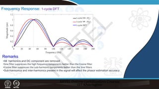
62. Frequency Response: 1-cycle DFT (8 points, 50 Hz signal)
Sample No. Delays Sin(-∆θ)
0 7 1.0 0
1 6
2 5 0 -1
3 4
4 3 -1 0
5 2
6 1 0 1
7 0
z-Transform of cosine filter
Hc(ω) =
1
4
[1.0𝑧𝑧7 +
1
2
𝑧𝑧6 + 0.0𝑧𝑧 −
1
2
𝑧𝑧4 − 1.0𝑧𝑧3 −
1
2
𝑧𝑧2 + 0.0𝑧𝑧1 +
1
2
𝑧𝑧0]
Hs(ω) =
1
4
[0.0𝑧𝑧7 −
1
2
𝑧𝑧6 − 1.0𝑧𝑧5 −
1
2
𝑧𝑧4 − 0.0𝑧𝑧3 +
1
2
𝑧𝑧2 + 1.0𝑧𝑧1 +
1
2
𝑧𝑧0]
Window N=8
∆θ =
2π𝑛𝑛
𝑁𝑁
̇
𝑉𝑉 =
2
𝑁𝑁
�
𝑛𝑛=0
𝑁𝑁−1
(𝑣𝑣𝑛𝑛𝑒𝑒−𝑗𝑗
2𝜋𝜋
𝑁𝑁
𝑛𝑛
)
50 Hz signal, Sampling rate 0.4 kHz, ∆t=0.0025 s
z-Transform of sine filter
N
P
T
E
L

63. • Frequency response of the filter can be obtained by substituting 𝑧𝑧 = 𝑒𝑒𝑗𝑗𝑗𝑗∆𝑡𝑡
Where ∆𝑡𝑡= sampling time interval and 𝜔𝜔=frequency of input signal.
Frequency Response: 1-cycle DFT
Cosine Filter
• For fundamental frequency input, 𝜔𝜔=2𝜋𝜋 x 50 = 100𝜋𝜋
𝐻𝐻𝑐𝑐 100𝜋𝜋 =
1
4
1.0
1
2
− 𝑗𝑗
1
2
+
1
2
0 − 𝑗𝑗𝑗 + 0.0 −
1
2
− 𝑗𝑗
1
2
−
1
2
−1 + 𝑗𝑗𝑗.0 −
1.0 −
1
2
+ 𝑗𝑗
1
2
−
1
2
0 + 𝑗𝑗𝑗 + 0.0
1
2
+ 𝑗𝑗
1
2
+
1
2
1 + 𝑗𝑗𝑗
=
1
4
4 ×
1
2
− 4 × 𝑗𝑗
1
2
=
1
2
− 𝑗𝑗
1
2
= 1∠ −
𝜋𝜋
4
N
P
T
E
L

64. 𝐻𝐻𝑠𝑠 100𝜋𝜋 =
1
4
[0.0
1
2
− 𝑗𝑗
1
2
−
1
2
0 − 𝑗𝑗1 − 1.0 −
1
2
− 𝑗𝑗
1
2
−
1
2
−1 + 𝑗𝑗0.0
Frequency Response: 1-cycle DFT
Sine Filter
N
P
T
E
L

65. Frequency Response: 1-cycle DFT
Power System Relaying Committee IEEE working group report, Understanding microprocessor based technology applied to relaying,
Feb2004
L. Wang, Frequency Response of Phasor based microprocessor relaying algorithms, IEEETransactions on Power Delivery, vol 14, no.1,
1999, page 98
 For DC component, 𝜔𝜔=0
Hc (0) =
1
4
1.0 +
1
2
+ 0.0 −
1
2
− 1.0 −
1
2
+ 0.0 +
1
2
= 0
Hs (0) =
1
4
[0.0 −
1
2
− 1.0 −
1
2
− 0.0 +
1
2
+ 1.0 +
1
2
] = 0
 For second harmonic, 𝜔𝜔=2𝜋𝜋 2 50 =200𝜋𝜋
Hc (200𝜋𝜋) =0
Hs (200𝜋𝜋) = 0
x x
N
P
T
E
L

66. Frequency Response: 1-cycle DFT
Remarks
•All harmonics and DC component are removed
•Sine filter suppresses the high frequency components better than the Cosine filter
•Cosine filter suppresses the sub-harmonic components better than the Sine filters
•Sub-harmonics and inter-harmonics present in the signal will affect the phasor estimation accuracy
COS
SIN
N
P
T
E
L

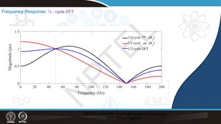
67. Frequency Response: ½ - cycle DFT
Sample No. Delays Sin(-∆θ)
0 3 1.0 0
1 2
2 1 0 -1
3 0
Using z-Transform
Hc(ω) =
1
4
[1.0𝑧𝑧3 +
1
2
𝑧𝑧2 + 0.0𝑧𝑧1 −
1
2
𝑧𝑧0]
Hs(ω) =
1
4
[0.0𝑧𝑧3 −
1
2
𝑧𝑧2 − 1.0𝑧𝑧1 −
1
2
𝑧𝑧0]
̇
𝑉𝑉 =
2
𝑁𝑁
2
�
𝑛𝑛=0
𝑁𝑁
2
−1
𝑣𝑣𝑛𝑛𝑒𝑒−𝑗𝑗
2𝜋𝜋
𝑁𝑁
𝑛𝑛
∆θ =
2π𝑛𝑛
𝑁𝑁
N
P
T
E
L

68. Frequency Response: ½ - cycle DFT
COS
SIN
N
P
T
E
L

69. Frequency Response: Least square technique- 1 cycle data window
N
P
T
E
L

70. Remarks-
• Frequency response shows – the rejection of filters to harmonics and DC–steady state
• One cycle DFT vs half cycle DFT
• Least square filter- with larger window
*******
N
P
T
E
L

71. Power System Protection
Prof A K Pradhan
Electrical Engineering, IIT KHARAGPUR
Module 02: Phasor Estimation
Lecture 10 : In the Presence of Decaying DC
N
P
T
E
L

72. Lecture 10: In the Presence of Decaying DC
• Decaying DC issue in the fault signals
• Solution
N
P
T
E
L

73. Presence of Decaying DC in current signal:
v(t)
R L
v t = V sin ωt + θ
i t = 𝐼𝐼𝑚𝑚[sin ωt + θ − θz − sin θ − θz e−
t
τ]
Here, θz = tan−1(
X
R
) =tan−1(
ωL
R
)
θ − θz = nπ ; zero transient, n=0,1,2,3..
θ − θz =
nπ
2
; maximum transient, n=1,3,5..
Thus, for different faults, fault inceptions, the relay will see different amount of decaying DC
The decaying DC will result in larger magnitude of phasor, leading to incorrect relay
decision
i t
N
P
T
E
L

74. Solution: Elimination of Decaying DC using Mimic Filter :
i(t)
R’ L’
Let decaying dc, i t = e−
t
τ
Vo s = sL′
+ R′
I s
ℒ−1 Vo(s) = ℒ−1[
sL′+R′
s+
1
τ
]
= L′
ℒ−1
s+
1
𝜏𝜏
s+
1
τ
= L′
u(t)
𝑤𝑤𝑤𝑤𝑤𝑤𝑤, 𝜏𝜏 =
L′
R′
Vo(t)
Mimic impedance where u(t)– unit impulse
 This implies, decaying DC in the output has vanished
N
P
T
E
L

75. Relay current with Mimic Filter
• Decaying DC is filtered out.
• This introduces phase lag, that has to be compensated for correct phasor estimation.
N
P
T
E
L

76. Elimination of Decaying DC using Digital Mimic Filter :
• With a mimic circuit consisting of R-L in impedance form K(1+sτ), then the exponentially decaying component at the output will
vanish, provided its time constant is equal to τ.
• The differentiator circuit, as with s-term, can be emulated by digital FIR filter: (1-z-1)
• The impedance can be represented as: K[(1+ τ) - τ z-1]
• K has to be set in such a way that, at rated frequency (50/60 Hz), the filter gain will be 1.
• The corresponding gain
f= 50/60 Hz
Gain(f) = |K[(1+ τ)- τ𝑒𝑒−𝑗𝑗𝑗𝑗∆𝑡𝑡
]| = 1
• Solving this equation for K, we obtain 𝐾𝐾2
=
1
1 + τ − τ cos 2𝜋𝜋/𝑁𝑁 2 + τ sin 2𝜋𝜋/𝑁𝑁 2
• Thus using mimic filter, the current sample at pth instant can be obtained as,
𝑖𝑖′ 𝑝𝑝 = 𝐾𝐾 1 + τ ∗ 𝑖𝑖 𝑝𝑝 − τ ∗ 𝑖𝑖(𝑝𝑝 − 1)
N = number of samples per cycle
N
P
T
E
L

77. Fault current response using Digital Mimic Filter with phase shift compensation:
𝜙𝜙𝑠𝑠𝑠 = tan−1
𝜏𝜏 sin ⁄
2𝜋𝜋 𝑁𝑁
1 + 𝜏𝜏 − 𝜏𝜏 cos ⁄
2𝜋𝜋 𝑁𝑁
Phase shift with mimic filter,
𝜏𝜏 = decaying time constant
N = number of samples per cycle
G. Benmouyal, "Removal of DC-offset in current waveforms using digital mimic filtering," IEEE Trans. Power Del., vol. 10, no. 2, pp. 621-630, April
1995.
Gain(f) = |K[(1+ τ)- τ𝑒𝑒−𝑗𝑗𝑗𝑗∆𝑡𝑡
]| = 1
N
P
T
E
L

78. Least Square Estimation in Presence of Decaying DC
𝐼𝐼, 𝜃𝜃, 𝑘𝑘0, τ are unknowns
𝑖𝑖𝑛𝑛 = 𝐼𝐼 sin 𝜔𝜔𝑡𝑡𝑛𝑛 + 𝜃𝜃 + 𝑘𝑘0𝑒𝑒−
𝑡𝑡𝑛𝑛
𝜏𝜏
𝑋𝑋1 = 𝐼𝐼 𝑐𝑐𝑐𝑐𝑐𝑐 𝜃𝜃, 𝑋𝑋2 = 𝐼𝐼 𝑠𝑠𝑠𝑠𝑠𝑠 𝜃𝜃,
𝑎𝑎n1 = sin(𝜔𝜔𝑡𝑡n), 𝑎𝑎n2 = cos(𝜔𝜔𝑡𝑡n),
From Taylor series expansion
𝑘𝑘0𝑒𝑒−
𝑡𝑡𝑛𝑛
𝜏𝜏 = 𝑘𝑘0 − 𝑘𝑘0
𝑡𝑡𝑛𝑛
𝜏𝜏
+ 𝑘𝑘0
𝑡𝑡𝑛𝑛
2
2!𝜏𝜏2 − … … … …
Neglecting higher order terms,
𝑘𝑘0𝑒𝑒−
𝑡𝑡𝑛𝑛
𝜏𝜏 = 𝑘𝑘0 − 𝑘𝑘0
𝑡𝑡𝑛𝑛
𝜏𝜏
Thus, 𝑖𝑖𝑛𝑛 = 𝐼𝐼 𝑠𝑠𝑠𝑠𝑠𝑠 𝜔𝜔𝑡𝑡n 𝑐𝑐𝑐𝑐𝑐𝑐 𝜃𝜃 + 𝐼𝐼 sin 𝜃𝜃 cos 𝜔𝜔𝑡𝑡n + 𝑘𝑘0 − 𝑘𝑘0
𝑡𝑡𝑛𝑛
𝜏𝜏
𝑋𝑋3 = 𝑘𝑘0, 𝑋𝑋4 =
𝑘𝑘0
𝜏𝜏
𝑎𝑎n3 = 1, 𝑎𝑎n4 = −𝑡𝑡n
𝑡𝑡𝑛𝑛 = 𝑛𝑛Δ𝑡𝑡; 0 ≤ 𝑛𝑛 ≤ 𝑁𝑁 − 1
𝑤𝑤𝑤𝑤𝑤𝑤𝑤𝑤𝑤 𝑖𝑖𝑛𝑛 is current sample at 𝑡𝑡𝑛𝑛
N
P
T
E
L

79. Least Square Estimation in Presence of Decaying DC
A =
sin 𝜔𝜔𝑡𝑡0 cos 𝜔𝜔𝑡𝑡0 1 −𝑡𝑡0
sin 𝜔𝜔𝑡𝑡1 cos 𝜔𝜔𝑡𝑡1 1 −𝑡𝑡1
⋮ ⋮ ⋮ ⋮
⋮ ⋮ ⋮ ⋮
sin 𝜔𝜔𝑡𝑡n cos 𝜔𝜔𝑡𝑡n 1 −𝑡𝑡n
𝑋𝑋 =
𝐼𝐼 𝑐𝑐𝑐𝑐𝑐𝑐 𝜃𝜃
𝐼𝐼 𝑠𝑠𝑠𝑠𝑠𝑠 𝜃𝜃
𝑘𝑘0
𝑘𝑘0
𝜏𝜏
𝑚𝑚 =
𝑖𝑖0
𝑖𝑖1
⋮
⋮
𝑖𝑖n
𝑋𝑋 = 𝐴𝐴𝑇𝑇𝐴𝐴 −1𝐴𝐴𝑇𝑇𝑚𝑚
𝐼𝐼 = 𝑋𝑋1
2
+ 𝑋𝑋2
2
Note, here I(rms) =
𝐼𝐼
2
𝜃𝜃 = tan−1
𝑋𝑋2
𝑋𝑋1
N
P
T
E
L

80. Least Square Estimation in the Presence of Decaying DC: Example
𝑖𝑖𝑛𝑛 = 100 sin 100𝜋𝜋𝑡𝑡𝑛𝑛 + 30° + 250 𝑒𝑒−
𝑡𝑡𝑛𝑛
40 ) (A), 𝑡𝑡𝑛𝑛 = 𝑛𝑛∆𝑡𝑡, where ∆𝑡𝑡=0.0025 s
𝑚𝑚 =
299.38
345.95
335.95
275.21
A =
sin 𝜔𝜔𝑡𝑡0 cos 𝜔𝜔𝑡𝑡0 1 −𝑡𝑡0
sin 𝜔𝜔𝑡𝑡1 cos 𝜔𝜔𝑡𝑡1 1 −𝑡𝑡1
sin 𝜔𝜔𝑡𝑡2 cos 𝜔𝜔𝑡𝑡2 1 −𝑡𝑡2
sin 𝜔𝜔𝑡𝑡3 cos 𝜔𝜔𝑡𝑡3 1 −𝑡𝑡3
=
0 1 1 0
1
2
1
2
1 −
1
8
1 0 1 −
1
4
1
2
−
1
2
1 −
3
8
Using first four sample points (half cycle),
𝑋𝑋 =
𝐼𝐼 𝑐𝑐𝑐𝑐𝑐𝑐 𝜃𝜃
𝐼𝐼 𝑠𝑠𝑠𝑠𝑠𝑠 𝜃𝜃
𝑘𝑘0
𝑘𝑘0
𝜏𝜏
From Least Square technique, 𝑋𝑋 = 𝐴𝐴𝑇𝑇𝐴𝐴 −1𝑚𝑚
= 100
𝑋𝑋 =
86.60
50.00
249.38
0.12
I = 𝑋𝑋1
2
+ 𝑋𝑋2
2
𝜃𝜃 = tan−1
𝑋𝑋2
𝑋𝑋1
= 300
(A)
= 86.62
+ 502
Estimated current
𝐼𝐼(𝑟𝑟𝑟𝑟𝑟𝑟) = 70.7(A)
Estimated current phasor = 70.7∠30° (A) This is the correct phasor.
N
P
T
E
L

81. Remarks
• Decaying DC will affect phasor values unless being filtered out-
affects relay performance like- distance relay underreach
• Mitigation-
 Mimic filter approach with DFT
• Least square Technique– in the modelling we can incorporate
*******
N
P
T
E
L