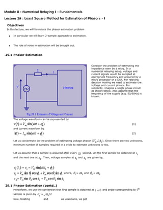
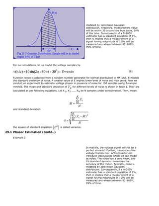
Module 8 : Numerical Relaying I : Fundamentals
Lecture 29 : Least Square Method for Estimation of Phasors - I
Objectives
In this lecture, we will formulate the phasor estimation problem
In particular we will learn 2-sample approach to estimation.
The role of noise in estimation will be brought out.
29.1 Phasor Estimation
Consider the problem of estimating the
impedance seen by a relay. In a
numerical relaying setup, voltage and
current signals would be sampled at
appropriate frequency and acquired by a
micro processor or a DSP. For relaying
decision making we need to estimate the
voltage and current phasor. For
simplicity, imagine a single phase circuit
as shown below. Also assume that the
frequency of the supply (e.g. 50/60Hz) is
known.
The voltage waveform can be represented by
(1)
and current waveform by
(2)
Let us concentrate on the problem of estimating voltage phasor ( ). Since there are two unknowns,
minimum number of samples required in a cycle to estimate unknowns is two.
Let us assume that a sample is acquired after every second. Let the first sample be obtained at
and the next one at . Then, voltage samples at and are given by,
where, and
29.1 Phasor Estimation (contd..)
Henceforth, we use the convention that first sample is obtained at and angle corresponding to jth
sample is given by
Now, treating and as unknowns, we get
(3)
(4)
and (5)
It is clear from eqns. (4) and (5) that if , m an integer, then , which
implies the singularity of coefficient matrix. In such an event, it is not possible to proceed with
estimation. For example, with , we get . Corresponding samples are shown in fig
29.2.
This corresponds to a sampling rate of two samples per cycle. If power system frequency is , this
implies that sampling rate should be higher than , so that . In fact, this is in agreement
with the well known sampling theorem (seen in previous lecture).
29.1 Phasor Estimation (contd..)
Henceforth, we use the convention that first sample is obtained at and angle corresponding to jth
sample is given by
Now, treating and as unknowns, we get
(3)
(4)
and (5)
It is clear from eqns. (4) and (5) that if , m an integer, then , which
implies the singularity of coefficient matrix. In such an event, it is not possible to proceed with
estimation. For example, with , we get . Corresponding samples are shown in fig
29.2.
This corresponds to a sampling rate of two samples per cycle. If power system frequency is , this
implies that sampling rate should be higher than , so that . In fact, this is in
agreement with the well known sampling theorem (seen in previous lecture).
29.1 Phasor Estimation (contd..)
Consequently and can be computed by following equations.
and
A generic form of the estimation is given by the following equation.
(6)
(7)
Infact, we have replaced the sample-2 by the most recent sample sample. Similarly sample-1 is
replaced by sample . We also say that sampling window has 2 samples per window (see fig 29.4).
In any relaying application, computations have to be completed before the arrival of next sample. Note
that, when uniform sampling is used with time space of sec. , a constant.
29.1 Phasor Estimation (contd..)
Example 1
Consider a signal , and a sampling time of 5 msec i.e. sampling rate 4
samples per cycle. Let the sampling be initiated at sec.
(a) Write down the sequence of first 10 voltage samples.
Ans: The sequence is summarized below.
t msec 0 5 10 15 20 25 30 35 40 45
V 5.00 8.66 -5.00 -8.66 5.00 8.66 -5.00 -8.66 5.00 8.66
(b) Compute the voltage phasor for 100 samples
Fig 29.3 shows the estimate of voltage magnitude as a function of samples. It is obvious that in the
absence of noise, estimate gives the right value of .
Fig 29.4 also introduces the concept of data window for estimation. This window contains the 'active' set
of samples which are currently being processed for phasor estimation. In the present case, we say that
we are using a 2-sample window. Each consecutive window, differs from the previous window by adding
a new sample and by removing the oldest active sample.
29.1 Phasor Estimation (contd..)
Example 2
In real life, the voltage signal will not be a
perfect sinusoid. Further, transducers like
voltage transformer, A/D converter etc.
introduce inaccuracies which we can model
as noise. The noise has a zero mean, and
it's standard deviation measures the
accuracy of the meter. Typically, noise is
modeled by zero mean Gaussian
distribution. Therefore, measurement value
will be within 36 around the true value, 99%
of the time. Consequently, if a 0-100V
voltmeter has a standard deviation of 1%,
then it implies that a measurement of a
signal having magnitude of 100V will be
measured any where between 97-103V,
99% of time.
For our simulations, let us model the voltage samples by
(8)
Function randn is obtained from a random number generator for normal distribution in MATLAB. E models
the standard deviation of noise. A smaller value of E implies lower level of noise and vice versa. Now we
conduct an experiment to estimate voltage phasor in presence of noise for 100 samples using 2-sample
method. The mean and standard deviation of for different levels of noise is shown in table 1. They are
calculated as per following equations. Let X1, X2 ..... XN be N samples under consideration. Then, mean
and standard deviation
the square of standard deviation is called variance.
29.1 Phasor Estimation (contd..)
Example 2
In real life, the voltage signal will not be a
perfect sinusoid. Further, transducers like
voltage transformer, A/D converter etc.
introduce inaccuracies which we can model
as noise. The noise has a zero mean, and
it's standard deviation measures the
accuracy of the meter. Typically, noise is
modeled by zero mean Gaussian
distribution. Consequently, if a 0-100V
voltmeter has a standard deviation of 1%,
then it implies that a measurement of a
signal having magnitude of 100V will be
measured any where between 97-103V,
99% of time.
For our simulations, let us model the voltage samples by
(8)
Function randn is obtained from a random number generator for normal distribution in MATLAB. E models
the standard deviation of noise. A smaller value of E implies lower level of noise and vice versa. Now we
conduct an experiment to estimate voltage phasor in presence of noise for 100 samples using 2-sample
method. The mean and standard deviation of for different levels of noise is shown in table 1. They are
calculated as per following equations. Let X1, X2 ..... XN be N samples under consideration. Then, mean
and standard deviation
the square of standard deviation is called variance.
29.1 Phasor Estimation (contd..)
Example 2
(contd..)
Table 1 : Effect of Gaussian Noise on Estimation of Phasors using 2-Sample Window
Randn multiplier(E) Mean Standard deviation
0.1 10.0069 0.1596
0.2 10.0162 0.3194
0.3 10.0282 0.4793
0.4 10.0426 0.6392
0.5 10.0596 0.7991
0.6 10.0791 0.9587
0.7 10.1011 1.1182
0.8 10.1256 1.2772
0.9 10.1527 1.4358
1.0 10.1824 1.5938
1.1 10.2146 1.7510
1.2 10.2495 1.9073
1.3 10.2871 2.0624
1.4 10.3275 2.2162
1.5 10.3707 2.3683
1.6 10.4169 2.5186
1.7 10.4662 2.6666
1.8 10.5188 2.8116
1.9 10.5750 2.9531
2.0 10.6346 3.0919
2.1 10.6975 3.2284
2.2 10.7638 3.3625
2.3 10.8336 3.4940
2.4 10.9065 3.6240
2.5 10.9825 3.7529
2.6 11.0613 3.8809
2.7 11.1430 4.0080
2.8 11.2277 4.1241
2.9 11.3152 4.2590
3.0 11.4055 4.3830
29.1 Phasor Estimation (contd..)
Example 2 (contd..)
Fig 29.6 shows the plot of estimated value of as a function of sample number for E = 0.5.
From fig 29.6 and table 1, it is evident that
1. As magnitude of zero mean noise increases, the standard deviation associated with magnitude increase.
2. Mean of is nearly 10.
3. Actual estimates seldom match with 10V.
This brings out an important fact that with bare minimum number of measurements, the noise affects the
accuracy. Therefore, in real-life, we have to device a procedure to filter noise and then estimate and
. To filter out noise, we need to consider redundant measurement. Redundancy in measurement is
defined as ratio of actual number of measurement used for estimation to minimum number of
measurement required for estimation. This issue is elaborated in the subsequent lecture.
Review Questions
1. Using MATLAB, repeat Example 1 and Example 2.
2. Derive two-sample estimation technique. Discuss it's limitation.
Recap
In this lecture we have learnt the following:
How to approach the phasor estimation problem in numerical relaying.
The significance of noise in estimation was brought out through 2-sample estimation method.

Lecture 29

  • 1.
    Module 8 :Numerical Relaying I : Fundamentals Lecture 29 : Least Square Method for Estimation of Phasors - I Objectives In this lecture, we will formulate the phasor estimation problem In particular we will learn 2-sample approach to estimation. The role of noise in estimation will be brought out. 29.1 Phasor Estimation Consider the problem of estimating the impedance seen by a relay. In a numerical relaying setup, voltage and current signals would be sampled at appropriate frequency and acquired by a micro processor or a DSP. For relaying decision making we need to estimate the voltage and current phasor. For simplicity, imagine a single phase circuit as shown below. Also assume that the frequency of the supply (e.g. 50/60Hz) is known. The voltage waveform can be represented by (1) and current waveform by (2) Let us concentrate on the problem of estimating voltage phasor ( ). Since there are two unknowns, minimum number of samples required in a cycle to estimate unknowns is two. Let us assume that a sample is acquired after every second. Let the first sample be obtained at and the next one at . Then, voltage samples at and are given by, where, and 29.1 Phasor Estimation (contd..) Henceforth, we use the convention that first sample is obtained at and angle corresponding to jth sample is given by Now, treating and as unknowns, we get
  • 2.
    (3) (4) and (5) It isclear from eqns. (4) and (5) that if , m an integer, then , which implies the singularity of coefficient matrix. In such an event, it is not possible to proceed with estimation. For example, with , we get . Corresponding samples are shown in fig 29.2. This corresponds to a sampling rate of two samples per cycle. If power system frequency is , this implies that sampling rate should be higher than , so that . In fact, this is in agreement with the well known sampling theorem (seen in previous lecture). 29.1 Phasor Estimation (contd..) Henceforth, we use the convention that first sample is obtained at and angle corresponding to jth sample is given by Now, treating and as unknowns, we get (3)
  • 3.
    (4) and (5) It isclear from eqns. (4) and (5) that if , m an integer, then , which implies the singularity of coefficient matrix. In such an event, it is not possible to proceed with estimation. For example, with , we get . Corresponding samples are shown in fig 29.2. This corresponds to a sampling rate of two samples per cycle. If power system frequency is , this implies that sampling rate should be higher than , so that . In fact, this is in agreement with the well known sampling theorem (seen in previous lecture). 29.1 Phasor Estimation (contd..) Consequently and can be computed by following equations. and A generic form of the estimation is given by the following equation. (6) (7)
  • 4.
    Infact, we havereplaced the sample-2 by the most recent sample sample. Similarly sample-1 is replaced by sample . We also say that sampling window has 2 samples per window (see fig 29.4). In any relaying application, computations have to be completed before the arrival of next sample. Note that, when uniform sampling is used with time space of sec. , a constant. 29.1 Phasor Estimation (contd..) Example 1 Consider a signal , and a sampling time of 5 msec i.e. sampling rate 4 samples per cycle. Let the sampling be initiated at sec. (a) Write down the sequence of first 10 voltage samples. Ans: The sequence is summarized below. t msec 0 5 10 15 20 25 30 35 40 45 V 5.00 8.66 -5.00 -8.66 5.00 8.66 -5.00 -8.66 5.00 8.66 (b) Compute the voltage phasor for 100 samples Fig 29.3 shows the estimate of voltage magnitude as a function of samples. It is obvious that in the absence of noise, estimate gives the right value of . Fig 29.4 also introduces the concept of data window for estimation. This window contains the 'active' set of samples which are currently being processed for phasor estimation. In the present case, we say that we are using a 2-sample window. Each consecutive window, differs from the previous window by adding a new sample and by removing the oldest active sample. 29.1 Phasor Estimation (contd..) Example 2 In real life, the voltage signal will not be a perfect sinusoid. Further, transducers like voltage transformer, A/D converter etc. introduce inaccuracies which we can model as noise. The noise has a zero mean, and it's standard deviation measures the accuracy of the meter. Typically, noise is
  • 5.
    modeled by zeromean Gaussian distribution. Therefore, measurement value will be within 36 around the true value, 99% of the time. Consequently, if a 0-100V voltmeter has a standard deviation of 1%, then it implies that a measurement of a signal having magnitude of 100V will be measured any where between 97-103V, 99% of time. For our simulations, let us model the voltage samples by (8) Function randn is obtained from a random number generator for normal distribution in MATLAB. E models the standard deviation of noise. A smaller value of E implies lower level of noise and vice versa. Now we conduct an experiment to estimate voltage phasor in presence of noise for 100 samples using 2-sample method. The mean and standard deviation of for different levels of noise is shown in table 1. They are calculated as per following equations. Let X1, X2 ..... XN be N samples under consideration. Then, mean and standard deviation the square of standard deviation is called variance. 29.1 Phasor Estimation (contd..) Example 2 In real life, the voltage signal will not be a perfect sinusoid. Further, transducers like voltage transformer, A/D converter etc. introduce inaccuracies which we can model as noise. The noise has a zero mean, and it's standard deviation measures the accuracy of the meter. Typically, noise is modeled by zero mean Gaussian distribution. Consequently, if a 0-100V voltmeter has a standard deviation of 1%, then it implies that a measurement of a signal having magnitude of 100V will be measured any where between 97-103V, 99% of time.
  • 6.
    For our simulations,let us model the voltage samples by (8) Function randn is obtained from a random number generator for normal distribution in MATLAB. E models the standard deviation of noise. A smaller value of E implies lower level of noise and vice versa. Now we conduct an experiment to estimate voltage phasor in presence of noise for 100 samples using 2-sample method. The mean and standard deviation of for different levels of noise is shown in table 1. They are calculated as per following equations. Let X1, X2 ..... XN be N samples under consideration. Then, mean and standard deviation the square of standard deviation is called variance. 29.1 Phasor Estimation (contd..) Example 2 (contd..) Table 1 : Effect of Gaussian Noise on Estimation of Phasors using 2-Sample Window Randn multiplier(E) Mean Standard deviation 0.1 10.0069 0.1596 0.2 10.0162 0.3194 0.3 10.0282 0.4793 0.4 10.0426 0.6392 0.5 10.0596 0.7991 0.6 10.0791 0.9587 0.7 10.1011 1.1182 0.8 10.1256 1.2772 0.9 10.1527 1.4358 1.0 10.1824 1.5938 1.1 10.2146 1.7510 1.2 10.2495 1.9073
  • 7.
    1.3 10.2871 2.0624 1.410.3275 2.2162 1.5 10.3707 2.3683 1.6 10.4169 2.5186 1.7 10.4662 2.6666 1.8 10.5188 2.8116 1.9 10.5750 2.9531 2.0 10.6346 3.0919 2.1 10.6975 3.2284 2.2 10.7638 3.3625 2.3 10.8336 3.4940 2.4 10.9065 3.6240 2.5 10.9825 3.7529 2.6 11.0613 3.8809 2.7 11.1430 4.0080 2.8 11.2277 4.1241 2.9 11.3152 4.2590 3.0 11.4055 4.3830 29.1 Phasor Estimation (contd..) Example 2 (contd..) Fig 29.6 shows the plot of estimated value of as a function of sample number for E = 0.5. From fig 29.6 and table 1, it is evident that 1. As magnitude of zero mean noise increases, the standard deviation associated with magnitude increase. 2. Mean of is nearly 10. 3. Actual estimates seldom match with 10V. This brings out an important fact that with bare minimum number of measurements, the noise affects the accuracy. Therefore, in real-life, we have to device a procedure to filter noise and then estimate and . To filter out noise, we need to consider redundant measurement. Redundancy in measurement is
  • 8.
    defined as ratioof actual number of measurement used for estimation to minimum number of measurement required for estimation. This issue is elaborated in the subsequent lecture. Review Questions 1. Using MATLAB, repeat Example 1 and Example 2. 2. Derive two-sample estimation technique. Discuss it's limitation. Recap In this lecture we have learnt the following: How to approach the phasor estimation problem in numerical relaying. The significance of noise in estimation was brought out through 2-sample estimation method.