This document discusses the discrete Fourier transform (DFT). The DFT is defined as the sum of a signal x[n] multiplied by complex exponentials with discrete frequencies. Specifically, the DFT X[k] of an N-point signal x[n] is defined as the sum from n=0 to N-1 of x[n] multiplied by e^(-j2πkn/N) for k from 0 to N-1. The inverse DFT approximates the original signal x[n] by summing X[k] multiplied by complex exponentials. The DFT allows analyzing signals in the frequency domain using a finite number of discrete frequencies, enabling digital signal processing on computers.

![5.2 c
J. Fessler, May 27, 2004, 13:14 (student version)
DTFT
FT
Sum shifted scaled replicates
Sum of shifted replicates
DTFS
Z
DFT
Sinc interpolation Rectangular window
Dirichlet interpolation
Rectangular window
Bandlimited: Time-limited:
Time-limited:
Bandlimited:
Sampling
Sampling
S
a
m
p
l
e
U
n
i
t
C
i
r
c
l
e
U
n
i
t
C
i
r
c
l
e
PSfrag replacements
x[n] = xa(nTs)
xa(t)
Xa(F)
x[n]
X(ω)
xps[n]
X[k]
X(z)
X[k] = X(ω)|ω= 2π
N k
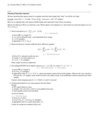
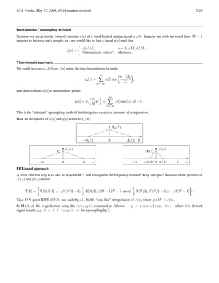
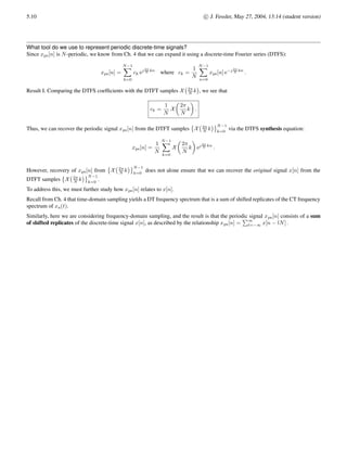
The FT Family Relationships
• FT
• Xa(F) =
R ∞
−∞
xa(t) e−2πF t
dt
• xa(t) =
R ∞
−∞
Xa(F) e2πF t
dF
• DTFT
• X(ω) =
P∞
n=−∞ x[n] e−ωn
= X(z)|z=ejω
• x[n] = 1
2π
R π
−π
X(ω) eωn
dω
• Uniform Time-Domain Sampling
• x[n] = xa(nTs)
• X(ω) = 1
Ts
P∞
k=−∞ Xa
ω/(2π)−k
Ts
(sum of shifted scaled replicates of Xa(·))
• Recovering xa(t) from x[n] for bandlimited xa(t), where Xa(F) = 0 for |F| ≥ Fs/2
• Xa(F) = Ts rect
F
Fs
X(2πFTs) (rectangular window to pick out center replicate)
• xa(t) =
P∞
n=−∞ x[n] sinc
t−nTs
Ts
, where sinc(x) = sin(πx) /(πx). (sinc interpolation)
• DTFS
• ck = 1
N
PN−1
n=0 xps[n] e− 2π
N kn
= 1
N X(z)|
z=e 2π
N
k
• xps[n] =
PN−1
k=0 ck e 2π
N kn
, ωk = 2π
N k
• Uniform Frequency-Domain Sampling
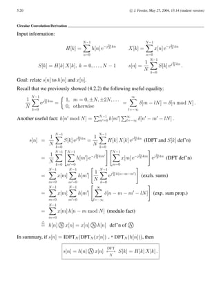
• X[k] = X(ω)](https://image.slidesharecdn.com/c5-220817121715-f46f998a/85/c5-pdf-2-320.jpg)
![ω= 2π
N k
, k = 0, . . . , N − 1
• X[k] = Nck
• xps[n] = 1
N
PN−1
k=0 X[k] e 2π
N kn
• xps[n] =
P∞
l=−∞ x[n − lN] (sum of shifted replicates of x[n])
• Recovering x[n] from X[k] for time-limited x[n], where x[n] = 0 except for n = 0, 1, . . . , L − 1 with L ≤ N
• x[n] = xps[n], n = 0, . . . , L − 1, 0 otherwise. (discrete-time rectangular window)
• X(ω) related to X[k] by Dirichlet interpolation: X(ω) =
PN−1
k=0 X[k] P(ω − 2πk/N), where P(ω) = 1
N
PN−1
k=0 e−ωn
.](https://image.slidesharecdn.com/c5-220817121715-f46f998a/85/c5-pdf-5-320.jpg)
![c
J. Fessler, May 27, 2004, 13:14 (student version) 5.3
Overview
Why yet another transform? After all, we now have FT tools for periodic and aperiodic signals in both CT and DT! What is left?
One of the most important properties of the DTFT is the convolution property: y[n] = h[n] ∗ x[n]
DTFT
↔ Y(ω) = H(ω) X(ω). This
property is useful for analyzing linear systems (and for filter design), and also useful for “on paper” convolutions of two sequences
h[n] and x[n], since if the sequences are simple ones whose DTFTs are known or are easily determined, we can simply multiply
the two transforms and then “look up” the inverse transform to get the convolution.
What if we want to automate this procedure using a computer? Right away there is a problem since ω is a continuous variable that
runs from −π to π, so it looks like we need an (uncountably) infinite number of ω’s which cannot be done on a computer.
For example, we cannot implement the ideal lowpass filter digitally.
This chapter exploit what happens if we do not use all the ω’s, but rather just a finite set (which can be stored digitally). In general
this will entail irrecoverable information loss. Fortunately, not always though! (Otherwise DSP would be a more academic subject.)
Any signal that is stored in a computer must be a finite length sequence, say x[0], x[1], . . . , x[L − 1] . Since there are only L signal
time samples, it stands to reason that we should not need an infinite number of frequencies to adequately represent the signal. In
fact, exactly N ≥ L frequencies should be enough information.
(We will see when we discuss zero-padding that for some purposes N ≈ 2L is an appropriate number of frequencies.)
Main points
• By the end of Chapter 5, we will know (among other things) how to use the DFT to convolve two generic sampled signals stored
in a computer. By the end of Ch. 6, we will know that by using the FFT, this approach to convolution is generally much faster
than using direct convolution, such as MATLAB’s conv command.
• Using the DFT via the FFT lets us do a FT (of a finite length signal) to examine signal frequency content. (This is how digital
spectrum analyzers work.)
Chapter 3 and 4 especially focussed on DT systems. Now we focus on DT signals for a while.
The discrete Fourier transform or DFT is the transform that deals with a finite discrete-time signal and a finite or discrete number
of frequencies.
Which frequencies?
ωk =
2π
N
k, k = 0, 1, . . . , N − 1.
For a signal that is time-limited to 0, 1, . . . , L − 1, the above N ≥ L frequencies contain all the information in the signal, i.e., we
can recover x[n] from
X 2π
N k
N−1
k=0
.
However, it is also useful to see what happens if we throw away all but those N frequencies even for general aperiodic signals.
Discrete-time Fourier transform (DTFT) review
Recall that for a general aperiodic signal x[n], the DTFT and its inverse is
X(ω) =
∞
X
n=−∞
x[n] e−ωn
, x[n] =
1
2π
Z π
−π
X(ω) eωn
dω .
Discrete-time Fourier series (DTFS) review
Recall that for a N-periodic signal x[n],
x[n] =
N−1
X
k=0
ck e 2π
N kn
where ck =
1
N
N−1
X
n=0
x[n] e− 2π
N kn
.](https://image.slidesharecdn.com/c5-220817121715-f46f998a/85/c5-pdf-6-320.jpg)
![5.4 c
J. Fessler, May 27, 2004, 13:14 (student version)
Definition(s)
The N-point DFT of any signal x[n] is defined as follows:
X[k]
4
=
PN−1
n=0 x[n] e− 2π
N kn
, k = 0, . . . , N − 1
?? otherwise.
Almost all books agree on the top part of this definition. (An exception is the 206 textbook (DSP First), which includes a 1
N out
front to make the DFT match the DTFS.)
But there are several possible choices for the “??” part of this definition.
1. Treat X[k] as an N-periodic function that is defined for all integer arguments k ∈ Z.
This is reasonable mathematically since
X[n + N] =
N−1
X
n=0
x[n] e− 2π
N (k+N)n
=
N−1
X
n=0
x[n] e−( 2π
N kn+2πkn)
=
N−1
X
n=0
x[n] e− 2π
N kn
= X[k] .
2. Treat X[k] as undefined for k /
∈ {0, . . . , N − 1}.
This is reasonable from a practical perspective since in a computer we have subroutines that take an N-point signal x[n]
and return only the N values X[0], . . . , X[N − 1], so trying to evaluate an expression like “X[−k]” will cause an error in a
computer.
3. Treat X[k] as being zero for k /
∈ {0, . . . , N − 1}.
This is a variation on the previous option.
The book seems to waver somewhat between the first two conventions.
These lecture notes are based on the middle convention: that the N-point DFT is undefined except for k ∈ {0, . . . , N − 1}. This
choice is made because it helps prevent computer programming errors.
Given X[k] for k ∈ {0, . . . , N − 1}, the N-point inverse DFT is defined as follows:
x̃[n] =
1
N
PN−1
k=0 X[k] e 2π
N kn
, n = 0, . . . , N − 1
??, otherwise.
Here the natural choice for the “??” part depends on the type of signal is under consideration.
• If x[n] is a finite length signal, supported on 0, . . . , L − 1, where L ≤ N, then we interpret the inverse DFT as
x[n] =
1
N
PN−1
k=0 X[k] e 2π
N kn
, n = 0, . . . , N − 1
0, otherwise.
This definition is the most important one since our primary use of the DFT is for length L signals with L ≤ N.
In this case the “inverse” is named appropriately, since we really do recover x[n] exactly from {X[k]}
N−1
k=0 . The proof of this is
essentially identical to the proof given for the self-consistency of the DTFS.
• If x[n] is a N-periodic signal, then we really should use the DTFS instead of the DFT, but they are so incredibly similar that
sometimes we will use the DFT, in which case we should interpret the inverse DFT as follows
x[n] =
1
N
N−1
X
k=0
X[k] e 2π
N kn
.
This is indeed a N-periodic expression.
• If x[n] is a signal whose length exceeds N, e.g., if x[n] is a aperiodic infinitely long signal, then the inverse DFT is best expressed
xps[n] =
1
N
N−1
X
k=0
X[k] e 2π
N kn
,
where xps[n] 6= x[n] in this case. (Nevertheless, it may be that xps[n] ≈ x[n] for n = 0, . . . , N − 1 so the DFT can be useful
even in this case.](https://image.slidesharecdn.com/c5-220817121715-f46f998a/85/c5-pdf-7-320.jpg)
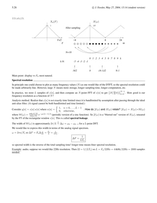
![c
J. Fessler, May 27, 2004, 13:14 (student version) 5.5
Examples
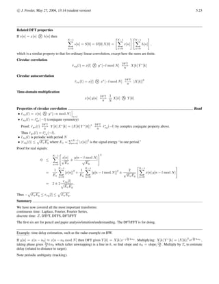
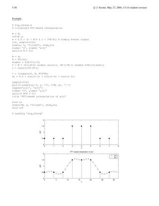
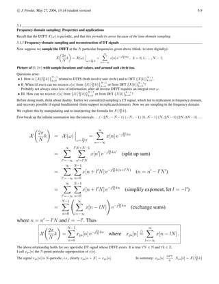
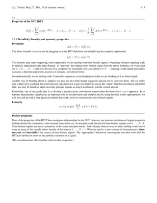
Example. x[n] = δ[n] +0.9 δ[n − 6]. What is L? L = 7. Let us use N = 8. (Powers of 2 are handy later for FFTs.)
X[k] =
N−1
X
n=0
x[n] e− 2π
N kn
=
7
X
n=0
x[n] e− 2π
8 kn
=
7
X
n=0
(δ[n] +0.9 δ[n − 6]) e−j2πkn/8
= 1 + 0.9 e− 2π
8 k6
.
0 1 2 3 4 5 6
−0.2
0
0.2
0.4
0.6
0.8
1
n
x[n]
DFT Example
0 1 2 3 4 5 6 7
0
0.5
1
1.5
2
k
|X[k]|
0 1 2 3 4 5 6 7
−1
−0.5
0
0.5
1
k
∠
X[k]
Alternative approach to finding X[k]. First find X(z), then sample around unit circle. X(z) = 1 + 0.9z−6
, so
X[k] = X(z)](https://image.slidesharecdn.com/c5-220817121715-f46f998a/85/c5-pdf-8-320.jpg)
![z=e 2π
N
k
= 1 + 0.9 e− 2π
8 k
.
Example. Find N-point inverse DFT of {X[k]}
N−1
k=0 where X[k] =
1, k = k0
0, otherwise
= δ[k − k0], for k0 ∈ {0, . . . , N − 1}.
Picture .
x[n] =
1
N
N−1
X
k=0
X[k] e 2π
N kn
=
1
N
e 2π
N k0n
.
Thus we have the following important DFT pair.
If k0 ∈ {0, . . . , N − 1} , then
1
N
e 2π
N k0n DFT
←→
N
δ[k − k0] .
Example. Find N-point inverse DFT of {X[k]}
N−1
k=0 where
X[k] =
eφ
, k = k0
e−φ
, k = N − k0
0, otherwise,
= eφ
δ[k − k0] + e−φ
δ[k − (N − k0])
for k0 ∈ {1, . . . , N/2 − 1, N/2 + 1, . . . , N − 1}. Picture .
x[n] =
1
N
N−1
X
k=0
X[k] e 2π
N kn
=
1
N
eφ
e 2π
N k0n
+
1
N
e−φ
e 2π
N (N−k0)n
=
2
N
cos
2π
N
k0n + φ
.](https://image.slidesharecdn.com/c5-220817121715-f46f998a/85/c5-pdf-11-320.jpg)
![5.6 c
J. Fessler, May 27, 2004, 13:14 (student version)
Example. Find the 8-point DFT of the signal x[n] = 6 cos2 π
4 n
.
Expanding: x[n] = 3 + 3 cos π
2 n
= 3 + 3
2 e 2π
8 2n
+ 3
2 e− 2π
8 2n
= 1
8
h
24 + 12 e 2π
8 2n
+ 12 e 2π
8 (8−2)n
i
.
So by coefficient matching, we see that X[k] = {24, 0, 12, 0, 0, 0, 12, 0} .
Example. Complex exponential signal with frequency that is an integer multiple of 2π
N .
Suppose x[n] = e 2π
N k0n
= eω0n
for n = 0, . . . , N − 1, where ω0 = 2π
N k0 and k0 is an integer.
Find the N-point DFT of x[n].
X[k] =
N−1
X
n=0
x[n] e− 2π
N kn
=
N−1
X
n=0
e 2π
N k0n
e− 2π
N kn
=
N−1
X
n=0
e− 2π
N (k−k0)n
=
N, k = k0 + lN, l ∈ Z
0, otherwise.
Thus
x[n] = e 2π
N k0n DFT
←→
N
X[k] = N
∞
X
l=−∞
δ[k − k0 − lN] = N δN [k − k0],
where δN [n]
4
=
P∞
l=−∞ δ[n − lN].
Example. Complex exponential signal with frequency that is not an integer multiple of 2π/N.
Suppose x[n] = eω0n
for n = 0, . . . , N − 1, where ω0 6= 2π
N k0 for any integer k.
Find the N-point DFT of x[n].
X[k] =
N−1
X
n=0
eω0n
e− 2π
N kn
=
N−1
X
n=0
e(ω0− 2π
N k)
n
=
1 −
e(ω0− 2π
N k)
N
1 − e(ω0− 2π
N k)
=
1 − eω0N
1 − e(ω0− 2π
N k)
.
Thus we have the following curious DFT pair.
If ω0/2π
N is non-integer, then eω0n DFT
←→
N
X[k] =
1 − eω0N
1 − e(ω0− 2π
N k)
.
What is going on in these examples?
Let s[n] = eω0n
be an eternal complex exponential signal, and define the following rectangular window
rN [n] =
1, n = 0, . . . , N − 1
0, otherwise,
which has the following DTFT:
R(ω) =
N−1
X
n=0
e−ωn
= · · · = e−ω(N−1)/2
Rr(ω), where Rr(ω) =
sin(ωN/2)
sin(ω/2)
, ω 6= 0
N, ω = 0
≈ N sinc
N
ω
2π
.
Then we have
x[n] = s[n] rN [n] =⇒ X(ω) = S(ω) ∗ RN (ω) = 2π δ(ω − ω0) ∗ R(ω) = 2π R(ω − ω0),
where the above δ is a Dirac impulse. Thus
X[k] = X(ω)](https://image.slidesharecdn.com/c5-220817121715-f46f998a/85/c5-pdf-12-320.jpg)

![c
J. Fessler, May 27, 2004, 13:14 (student version) 5.7
DTFT sampling preview
The DTFT formula is X(ω) =
P∞
n=−∞ x[n] e−ωn
whereas the DFT analysis formula is X[k] =
PN−1
n=0 x[n] e− 2π
N kn
.
If x[n] is a L-point signal, i.e., it is nonzero only for n = 0, 1, . . . , L−1, then the DTFT “simplifies” to X(ω) =
PL−1
n=0 x[n] e−ωn
.
Comparing these two formulas leads to the following conclusion.
If x[n] is a L-point signal with L ≤ N, then the N-point DFT values are samples of the DTFT:
X[k] = X(ω)](https://image.slidesharecdn.com/c5-220817121715-f46f998a/85/c5-pdf-16-320.jpg)

![ω= 2π
N k
.
If we are given a DTFT X(ω), and wish to find x[n], then the “usual” approach would be to apply the inverse DTFT, i.e., the DTFT
synthesis formula: x[n] = 1
2π
R π
−π
X(ω) eωn
dω .
However, performing this integral can be inconvenient.
The above relationship between the DFT and the DTFT suggests the following easier approach.
• First sample the DTFT X(ω) to get DFT values X[k], k = 0, . . . , N − 1.
• Then take the inverse DFT of X[k] (using the inverse FFT) to get (hopefully) the signal x[n].
Does this approach always work? No!
Why not? Because the DFT/DTFT relationship holds only if x[n] is an L-point signal with L ≤ N.
Example. Find the signal x[n] that has the following spectrum, with ω0 = π/2.
X(ω) =
3
4 −](https://image.slidesharecdn.com/c5-220817121715-f46f998a/85/c5-pdf-19-320.jpg)