Sanjivani Rural EducationSociety’s
Sanjivani College of Engineering, Kopargaon-423 603
(An Autonomous Institute, Affiliated to Savitribai Phule Pune University, Pune)
NACC ‘A’ Grade Accredited, ISO 9001:2015 Certified
Department of Computer Engineering
(NBA Accredited)
Prof. S. A. Shivarkar
Assistant Professor
Contact No.8275032712
Email- shivarkarsandipcomp@sanjivani.org.in
Subject- Supervised Modeling and AI Technologies (CO9401)
Unit –I: Supervised Learning Naïve Bayes and K-NN
2.
Content
Baysian classifier,Naive Bayes classifier cases, Constraints of Naïve bayes,
Advantages of Naïve Bayes, Comparison of Naïve bayes with other
classifiers,
K-nearest neighbor classifier, K-nearest neighbor classifier selection criteria,
Constraints of K-nearest neighbor, Advantages and Disadvantages of K-
nearest neighbor algorithms, controlling complexity of K-NN.
3.
Supervised vs. UnsupervisedLearning
Supervised learning (classification)- Prediction either Yes or No
Supervision: The training data (observations, measurements, etc.) are
accompanied by labels indicating the class of the observations.
New data is classified based on the training set.
Unsupervised learning (clustering)
The class labels of training data is unknown.
Given a set of measurements, observations, etc. with the aim of
establishing the existence of classes or clusters in the data.
4.
Prediction Problems: Classificationvs. Numeric Prediction
Classification
Predicts categorical class labels (discrete or nominal)
classifies data (constructs a model) based on the training set and the
values (class labels) in a classifying attribute and uses it in classifying new
data.
Numeric Prediction
Models continuous-valued functions, i.e., predicts unknown or missing
values .
Typical applications
Credit/loan approval: Loan approved Yes or No
Medical diagnosis: if a tumor is cancerous or benign
Fraud detection: if a transaction is fraudulent
Web page categorization: which category it is
5.
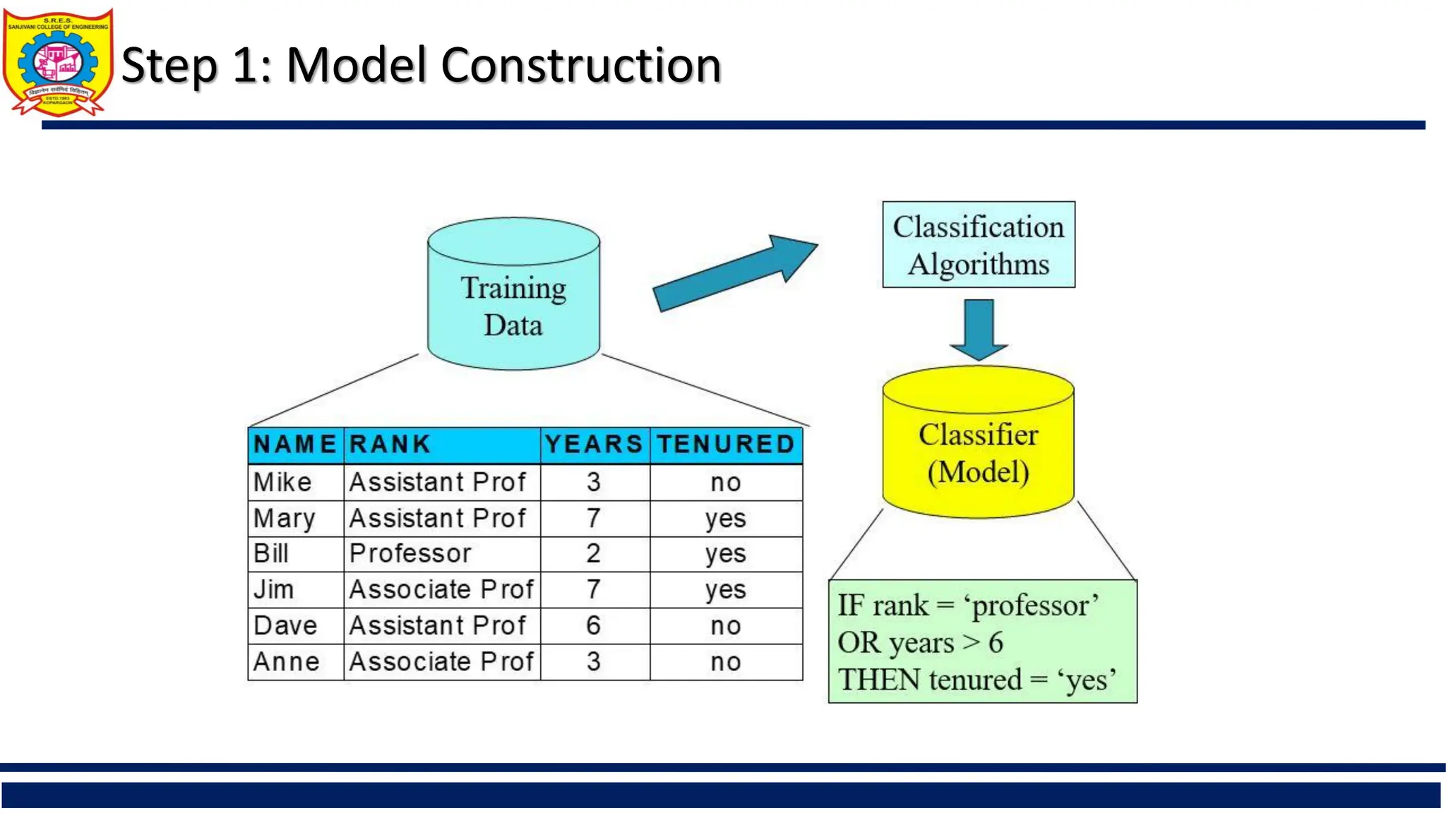
Classification—A Two-Step Process
Model construction: describing a set of predetermined classes
Each tuple/sample is assumed to belong to a predefined class, as determined by the class
label attribute
The set of tuples used for model construction is training set
The model is represented as classification rules, decision trees, or mathematical formulae
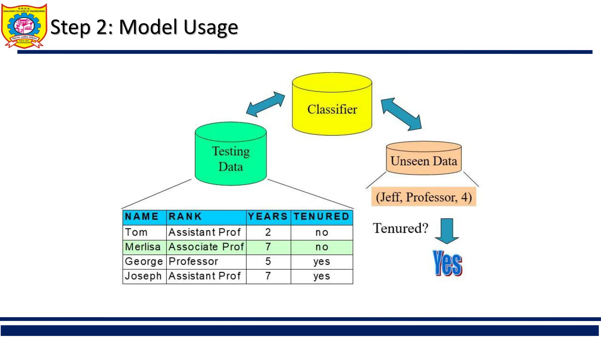
Model usage: for classifying future or unknown objects
Estimate accuracy of the model
The known label of test sample is compared with the classified result from the model
Accuracy rate is the percentage of test set samples that are correctly classified by the
model
Test set is independent of training set (otherwise overfitting)
If the accuracy is acceptable, use the model to classify new data
Note: If the test set is used to select models, it is called validation (test) set
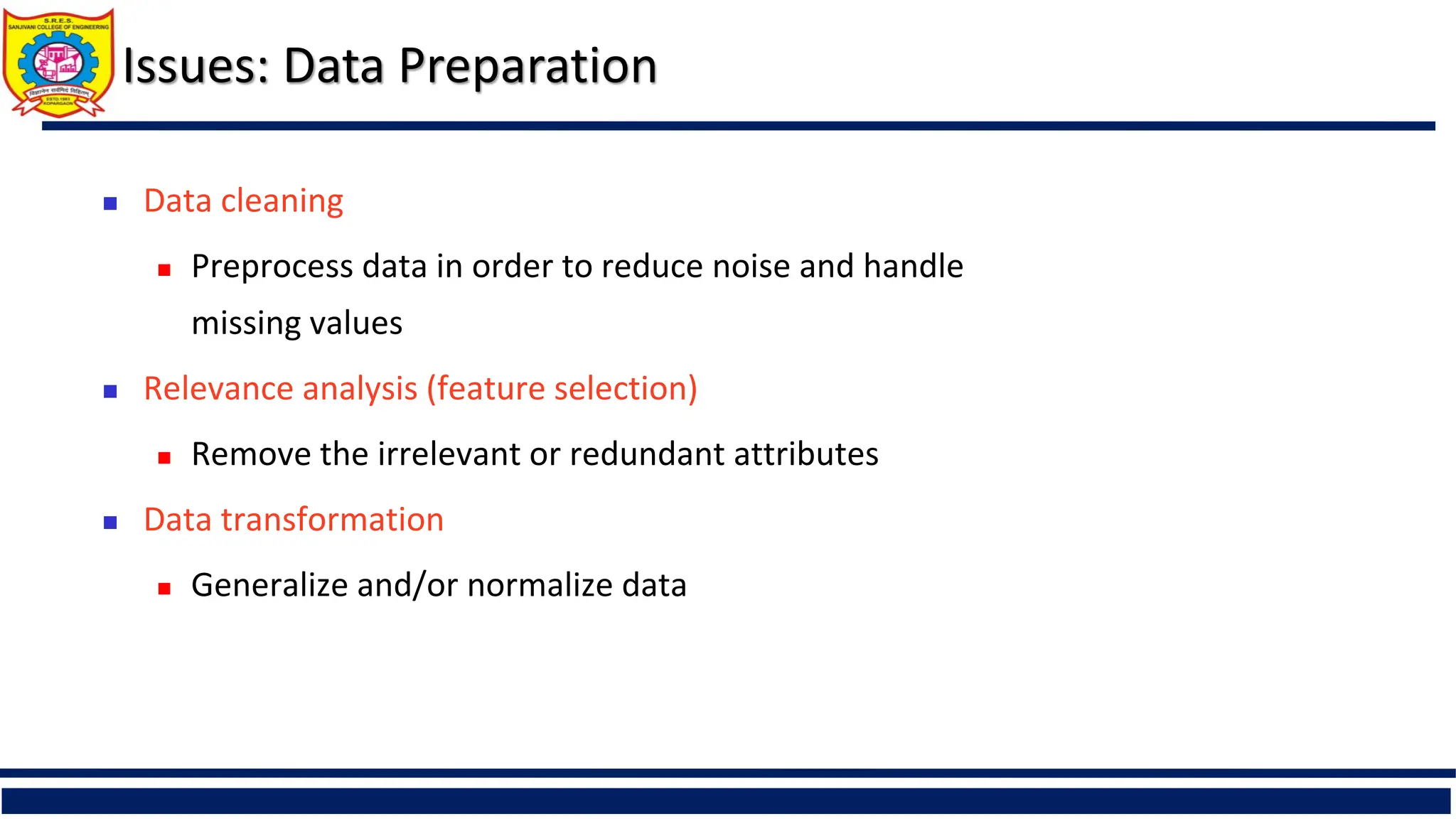
Issues: Data Preparation
Data cleaning
Preprocess data in order to reduce noise and handle
missing values
Relevance analysis (feature selection)
Remove the irrelevant or redundant attributes
Data transformation
Generalize and/or normalize data
9.
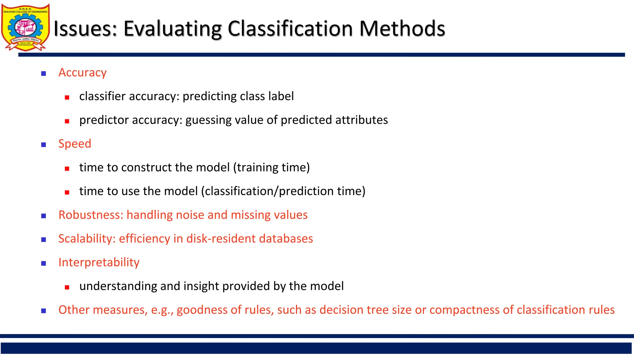
Issues: Evaluating ClassificationMethods
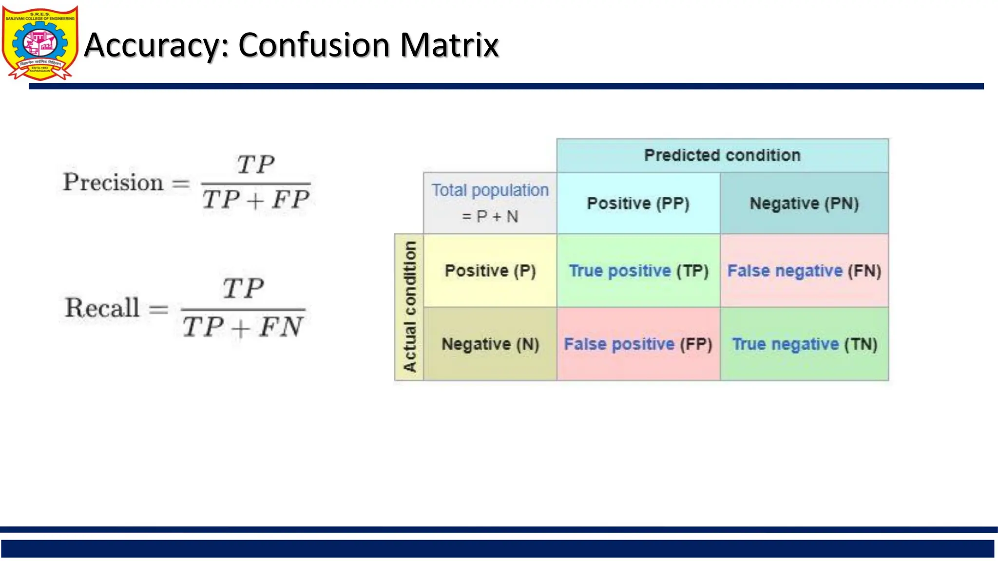
Accuracy
classifier accuracy: predicting class label
predictor accuracy: guessing value of predicted attributes
Speed
time to construct the model (training time)
time to use the model (classification/prediction time)
Robustness: handling noise and missing values
Scalability: efficiency in disk-resident databases
Interpretability
understanding and insight provided by the model
Other measures, e.g., goodness of rules, such as decision tree size or compactness of classification rules
10.
Issues: Evaluating ClassificationMethods: Accuracy
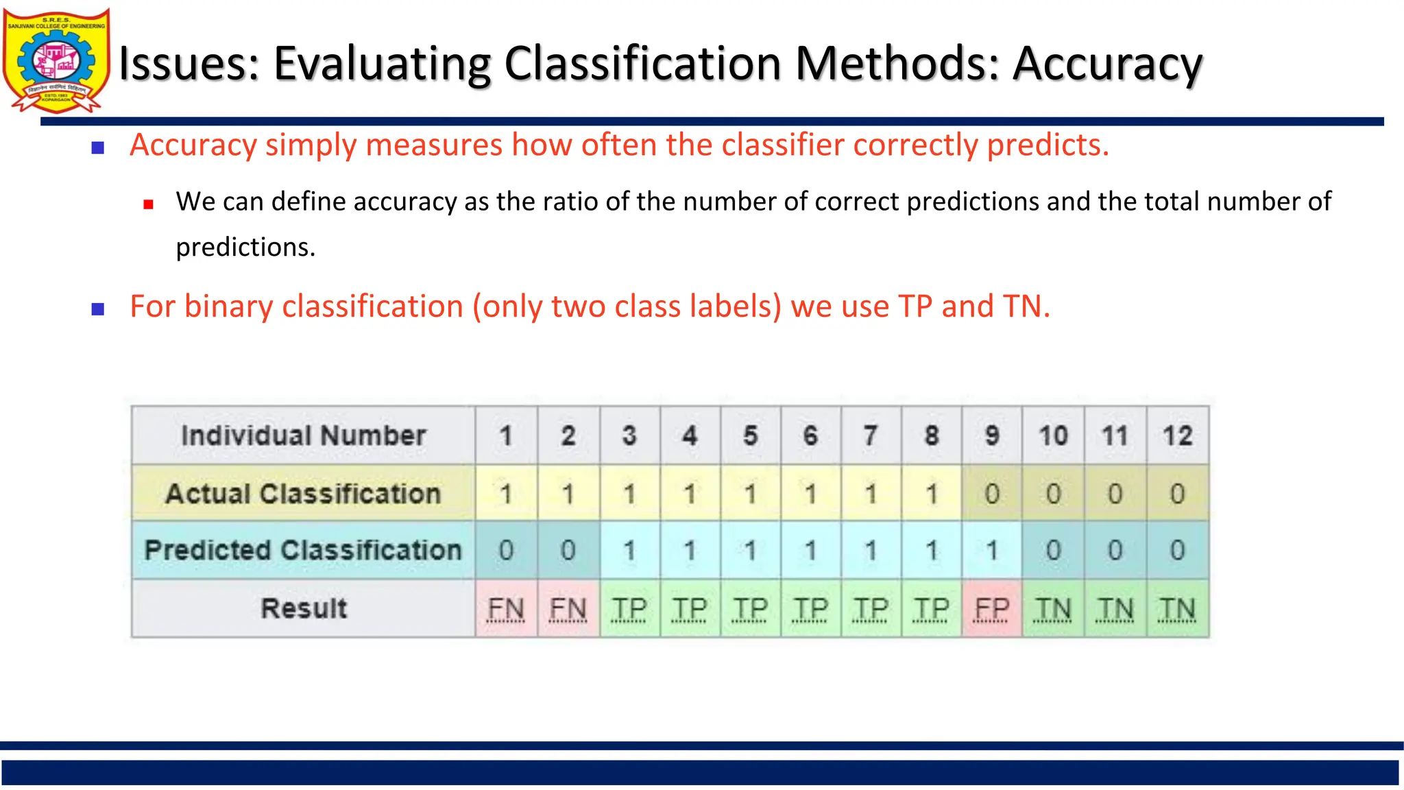
Accuracy simply measures how often the classifier correctly predicts.
We can define accuracy as the ratio of the number of correct predictions and the total number of
predictions.
For binary classification (only two class labels) we use TP and TN.
Bayesian Classification: Why?
A statistical classifier: performs probabilistic prediction, i.e., predicts class
membership probabilities
Foundation: Based on Bayes’ Theorem.
Performance: A simple Bayesian classifier, naïve Bayesian classifier, has comparable
performance with decision tree and selected neural network classifiers
Incremental: Each training example can incrementally increase/decrease the
probability that a hypothesis is correct — prior knowledge can be combined with
observed data
Standard: Even when Bayesian methods are computationally intractable, they can
provide a standard of optimal decision making against which other methods can be
measured
13.
Bayes’ Theorem: Basics
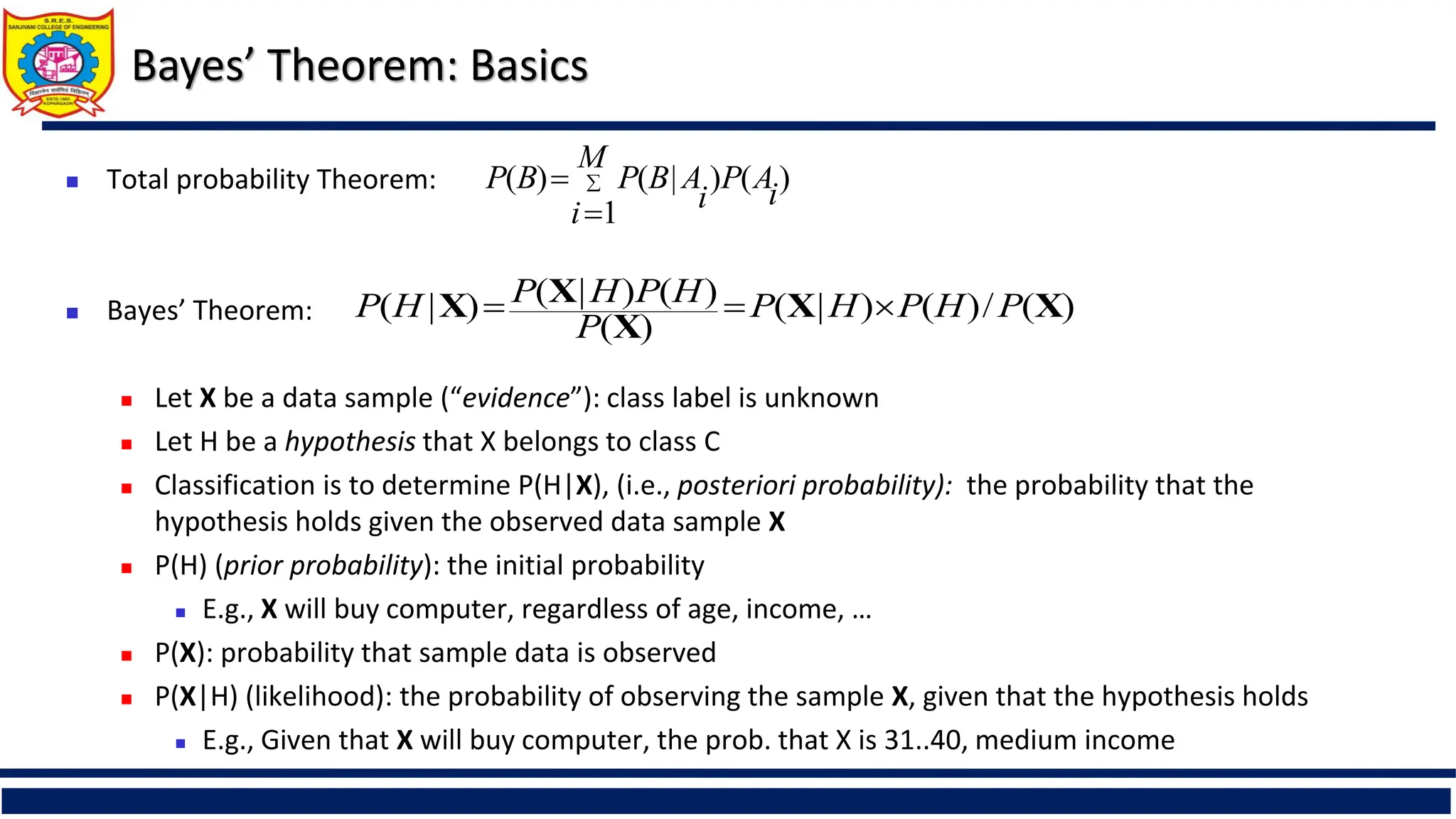
Total probability Theorem:
Bayes’ Theorem:
Let X be a data sample (“evidence”): class label is unknown
Let H be a hypothesis that X belongs to class C
Classification is to determine P(H|X), (i.e., posteriori probability): the probability that the
hypothesis holds given the observed data sample X
P(H) (prior probability): the initial probability
E.g., X will buy computer, regardless of age, income, …
P(X): probability that sample data is observed
P(X|H) (likelihood): the probability of observing the sample X, given that the hypothesis holds
E.g., Given that X will buy computer, the prob. that X is 31..40, medium income
)
(
)
1
|
(
)
( i
A
P
M
i i
A
B
P
B
P
)
(
/
)
(
)
|
(
)
(
)
(
)
|
(
)
|
( X
X
X
X
X P
H
P
H
P
P
H
P
H
P
H
P
14.
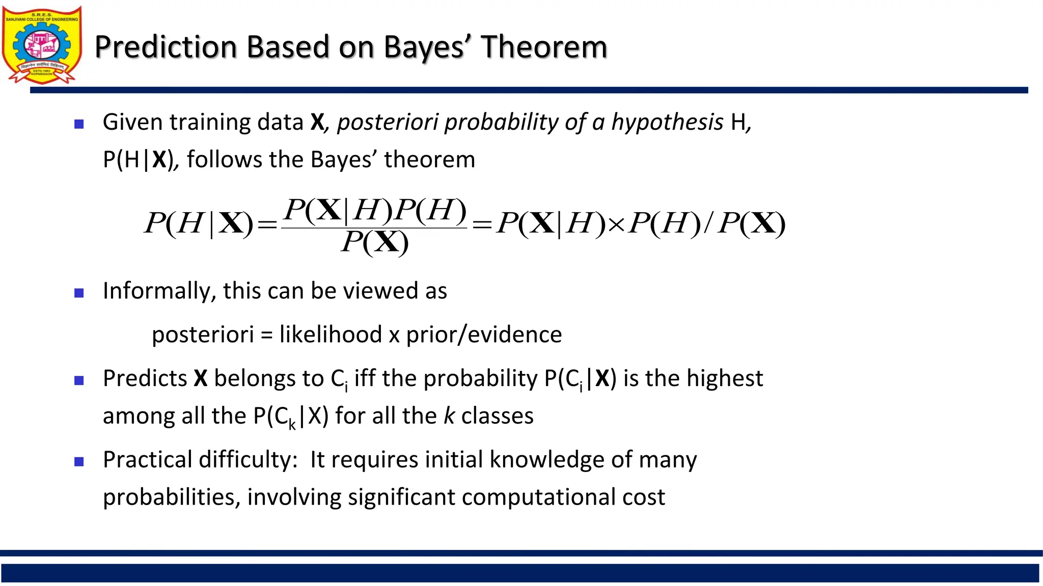
Prediction Based onBayes’ Theorem
Given training data X, posteriori probability of a hypothesis H,
P(H|X), follows the Bayes’ theorem
Informally, this can be viewed as
posteriori = likelihood x prior/evidence
Predicts X belongs to Ci iff the probability P(Ci|X) is the highest
among all the P(Ck|X) for all the k classes
Practical difficulty: It requires initial knowledge of many
probabilities, involving significant computational cost
)
(
/
)
(
)
|
(
)
(
)
(
)
|
(
)
|
( X
X
X
X
X P
H
P
H
P
P
H
P
H
P
H
P
15.
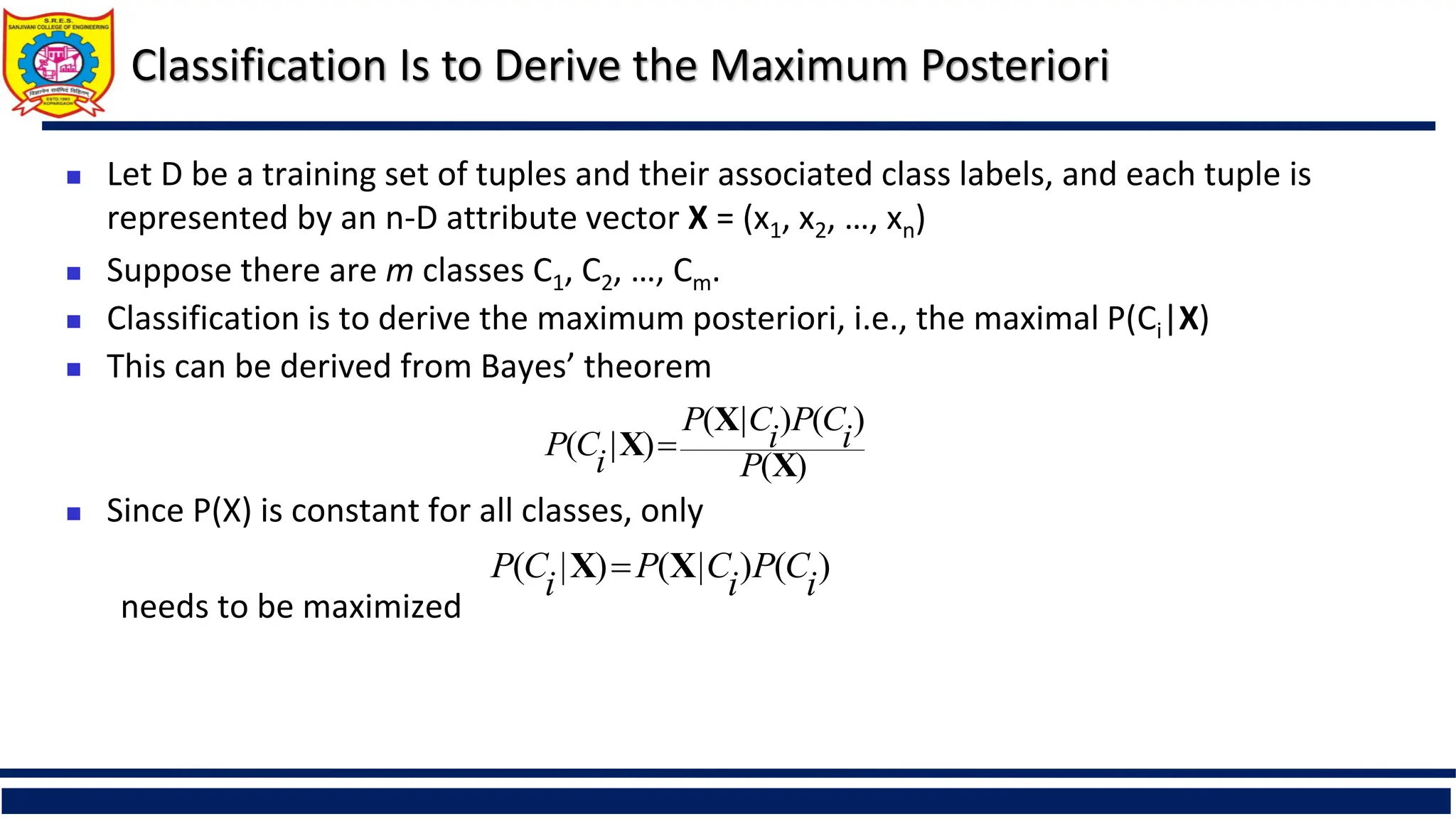
Classification Is toDerive the Maximum Posteriori
Let D be a training set of tuples and their associated class labels, and each tuple is
represented by an n-D attribute vector X = (x1, x2, …, xn)
Suppose there are m classes C1, C2, …, Cm.
Classification is to derive the maximum posteriori, i.e., the maximal P(Ci|X)
This can be derived from Bayes’ theorem
Since P(X) is constant for all classes, only
needs to be maximized
)
(
)
(
)
|
(
)
|
(
X
X
X
P
i
C
P
i
C
P
i
C
P
)
(
)
|
(
)
|
( i
C
P
i
C
P
i
C
P X
X
16.
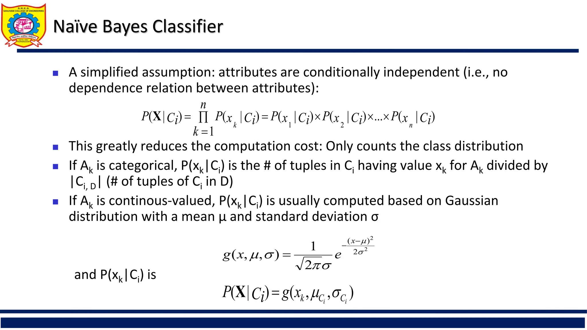
Naïve Bayes Classifier
A simplified assumption: attributes are conditionally independent (i.e., no
dependence relation between attributes):
This greatly reduces the computation cost: Only counts the class distribution
If Ak is categorical, P(xk|Ci) is the # of tuples in Ci having value xk for Ak divided by
|Ci, D| (# of tuples of Ci in D)
If Ak is continous-valued, P(xk|Ci) is usually computed based on Gaussian
distribution with a mean μ and standard deviation σ
and P(xk|Ci) is
)
|
(
...
)
|
(
)
|
(
1
)
|
(
)
|
(
2
1
Ci
x
P
Ci
x
P
Ci
x
P
n
k
Ci
x
P
Ci
P
n
k
X
2
2
2
)
(
2
1
)
,
,
(
x
e
x
g
)
,
,
(
)
|
( i
i C
C
k
x
g
Ci
P
X
17.
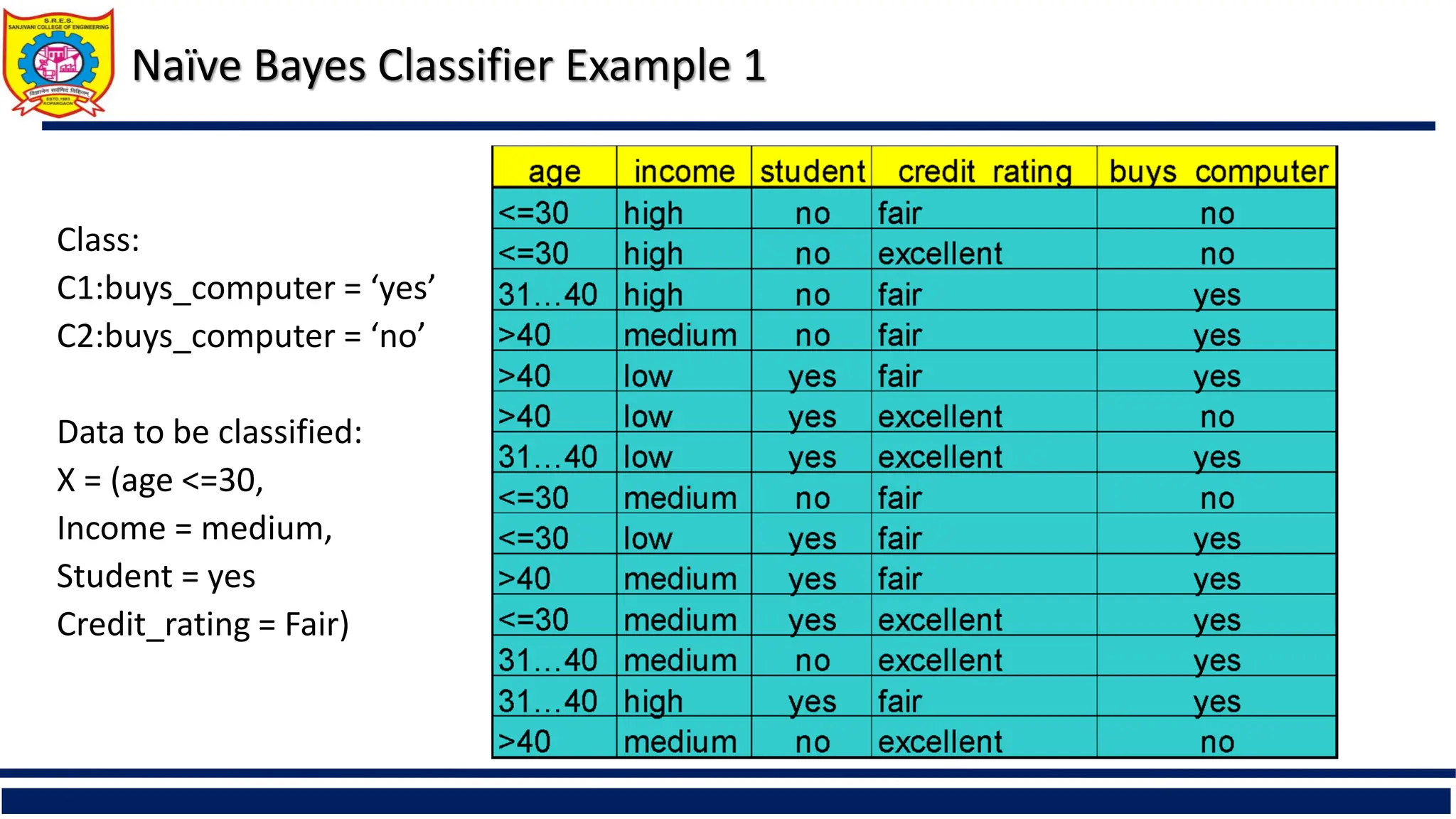
Naïve Bayes ClassifierExample 1
Class:
C1:buys_computer = ‘yes’
C2:buys_computer = ‘no’
Data to be classified:
X = (age <=30,
Income = medium,
Student = yes
Credit_rating = Fair)
18.
Naïve Bayes ClassifierExample 1 Solution
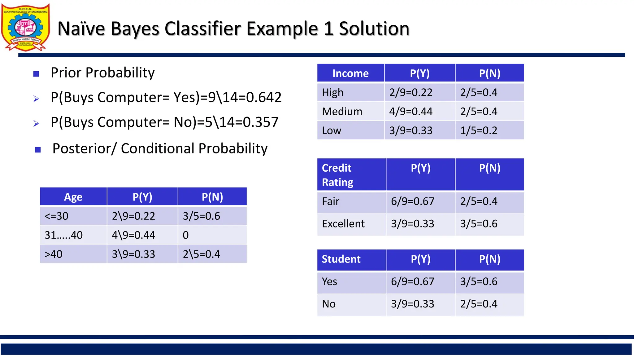
Age P(Y) P(N)
<=30 29=0.22 3/5=0.6
31…..40 49=0.44 0
>40 39=0.33 25=0.4
Prior Probability
P(Buys Computer= Yes)=914=0.642
P(Buys Computer= No)=514=0.357
Posterior/ Conditional Probability
Income P(Y) P(N)
High 2/9=0.22 2/5=0.4
Medium 4/9=0.44 2/5=0.4
Low 3/9=0.33 1/5=0.2
Credit
Rating
P(Y) P(N)
Fair 6/9=0.67 2/5=0.4
Excellent 3/9=0.33 3/5=0.6
Student P(Y) P(N)
Yes 6/9=0.67 3/5=0.6
No 3/9=0.33 2/5=0.4
19.
Naïve Bayes ClassifierExample 1 Solution
Age P(Y) P(N)
<=30 29=0.22 3/5=0.6
31…..40 49=0.44 0
>40 39=0.33 25=0.4
Prior Probability
P(Buys Computer= Yes)=914=0.642
P(Buys Computer= No)=514=0.357
Posterior/ Conditional Probability
Income P(Y) P(N)
High 2/9=0.22 2/5=0.4
Medium 4/9=0.44 2/5=0.4
Low 3/9=0.33 1/5=0.2
Credit
Rating
P(Y) P(N)
Fair 6/9=0.67 2/5=0.4
Excellent 3/9=0.33 3/5=0.6
Student P(Y) P(N)
Yes 6/9=0.67 3/5=0.6
No 3/9=0.33 2/5=0.4
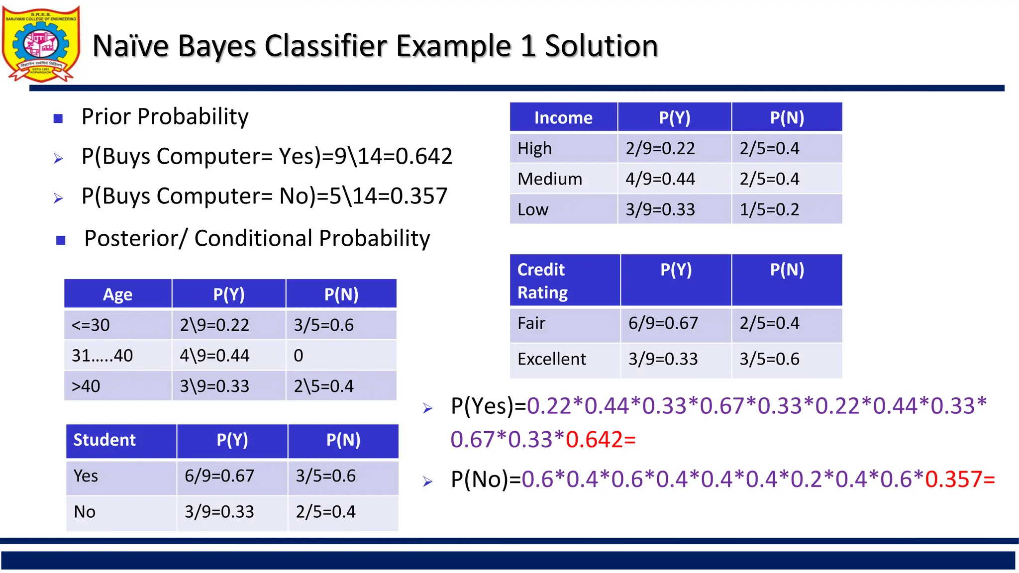
P(Yes)=0.22*0.44*0.33*0.67*0.33*0.22*0.44*0.33*
0.67*0.33*0.642=
P(No)=0.6*0.4*0.6*0.4*0.4*0.4*0.2*0.4*0.6*0.357=
20.
Naïve Bayes ClassifierExample 1 Solution
Age P(Y) P(N)
<=30 29=0.22 3/5=0.6
31…..40 49=0.44 0
>40 39=0.33 25=0.4
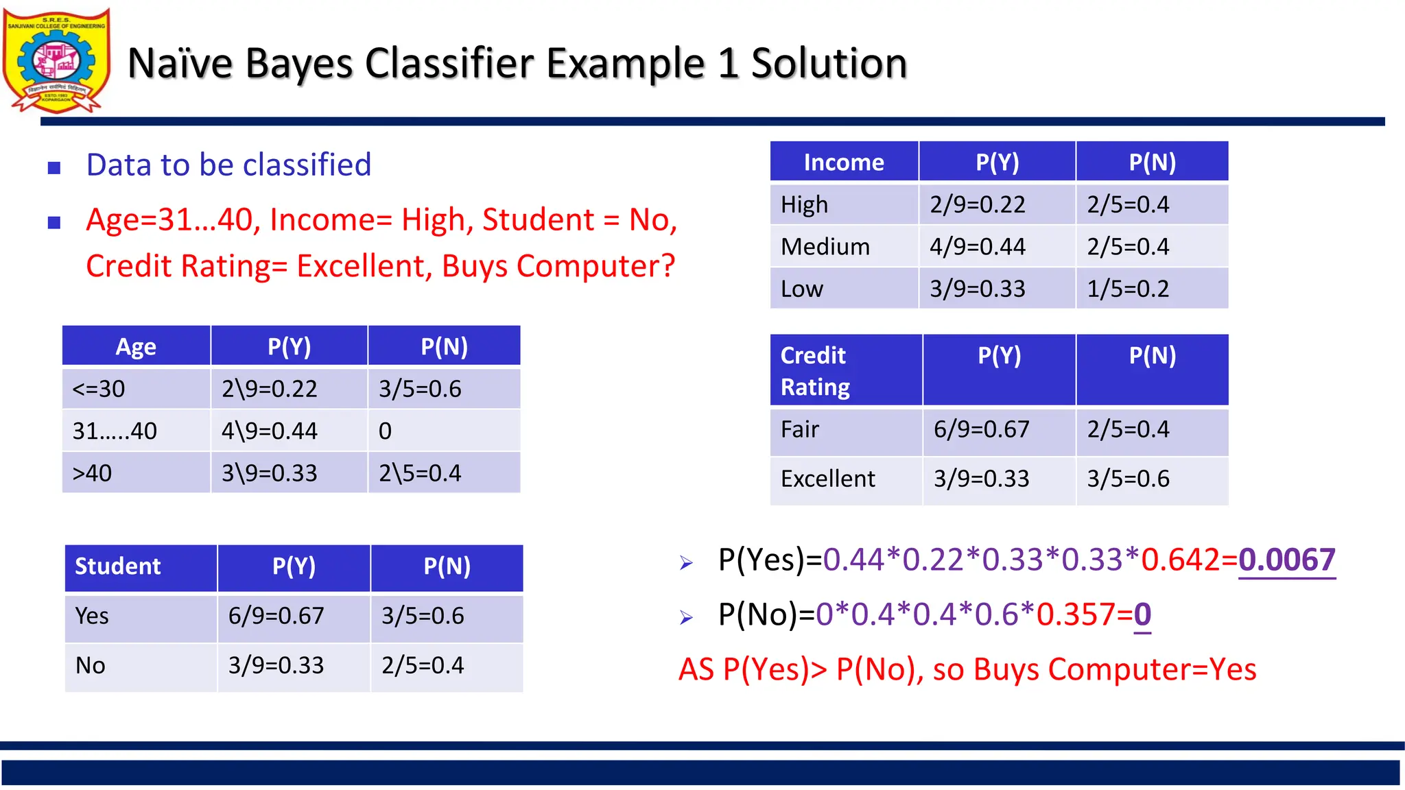
Data to be classified
Age=31…40, Income= High, Student = No,
Credit Rating= Excellent, Buys Computer?
Income P(Y) P(N)
High 2/9=0.22 2/5=0.4
Medium 4/9=0.44 2/5=0.4
Low 3/9=0.33 1/5=0.2
Credit
Rating
P(Y) P(N)
Fair 6/9=0.67 2/5=0.4
Excellent 3/9=0.33 3/5=0.6
Student P(Y) P(N)
Yes 6/9=0.67 3/5=0.6
No 3/9=0.33 2/5=0.4
P(Yes)=0.44*0.22*0.33*0.33*0.642=0.0067
P(No)=0*0.4*0.4*0.6*0.357=0
AS P(Yes)> P(No), so Buys Computer=Yes
21.
Naïve Bayes ClassifierExample 2
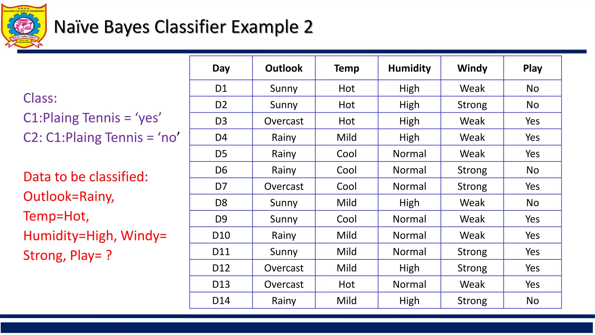
Class:
C1:Plaing Tennis = ‘yes’
C2: C1:Plaing Tennis = ‘no’
Data to be classified:
Outlook=Rainy,
Temp=Hot,
Humidity=High, Windy=
Strong, Play= ?
Day Outlook Temp Humidity Windy Play
D1 Sunny Hot High Weak No
D2 Sunny Hot High Strong No
D3 Overcast Hot High Weak Yes
D4 Rainy Mild High Weak Yes
D5 Rainy Cool Normal Weak Yes
D6 Rainy Cool Normal Strong No
D7 Overcast Cool Normal Strong Yes
D8 Sunny Mild High Weak No
D9 Sunny Cool Normal Weak Yes
D10 Rainy Mild Normal Weak Yes
D11 Sunny Mild Normal Strong Yes
D12 Overcast Mild High Strong Yes
D13 Overcast Hot Normal Weak Yes
D14 Rainy Mild High Strong No
22.
Naïve Bayes ClassifierExample 2 Solution
Outlook P(Y) P(N)
Sunny 29=0.22 3/5=0.6
Overcast 49=0.44 0
Rainy 39=0.33 25=0.4
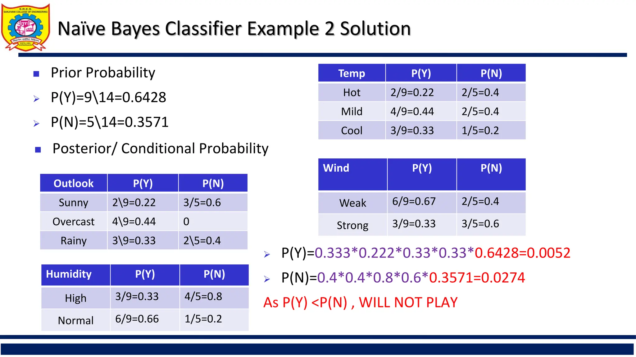
Prior Probability
P(Y)=914=0.6428
P(N)=514=0.3571
Posterior/ Conditional Probability
Temp P(Y) P(N)
Hot 2/9=0.22 2/5=0.4
Mild 4/9=0.44 2/5=0.4
Cool 3/9=0.33 1/5=0.2
Wind P(Y) P(N)
Weak 6/9=0.67 2/5=0.4
Strong 3/9=0.33 3/5=0.6
Humidity P(Y) P(N)
High 3/9=0.33 4/5=0.8
Normal 6/9=0.66 1/5=0.2
P(Y)=0.333*0.222*0.33*0.33*0.6428=0.0052
P(N)=0.4*0.4*0.8*0.6*0.3571=0.0274
As P(Y) <P(N) , WILL NOT PLAY
23.
Naïve Bayes ClassifierExample 3
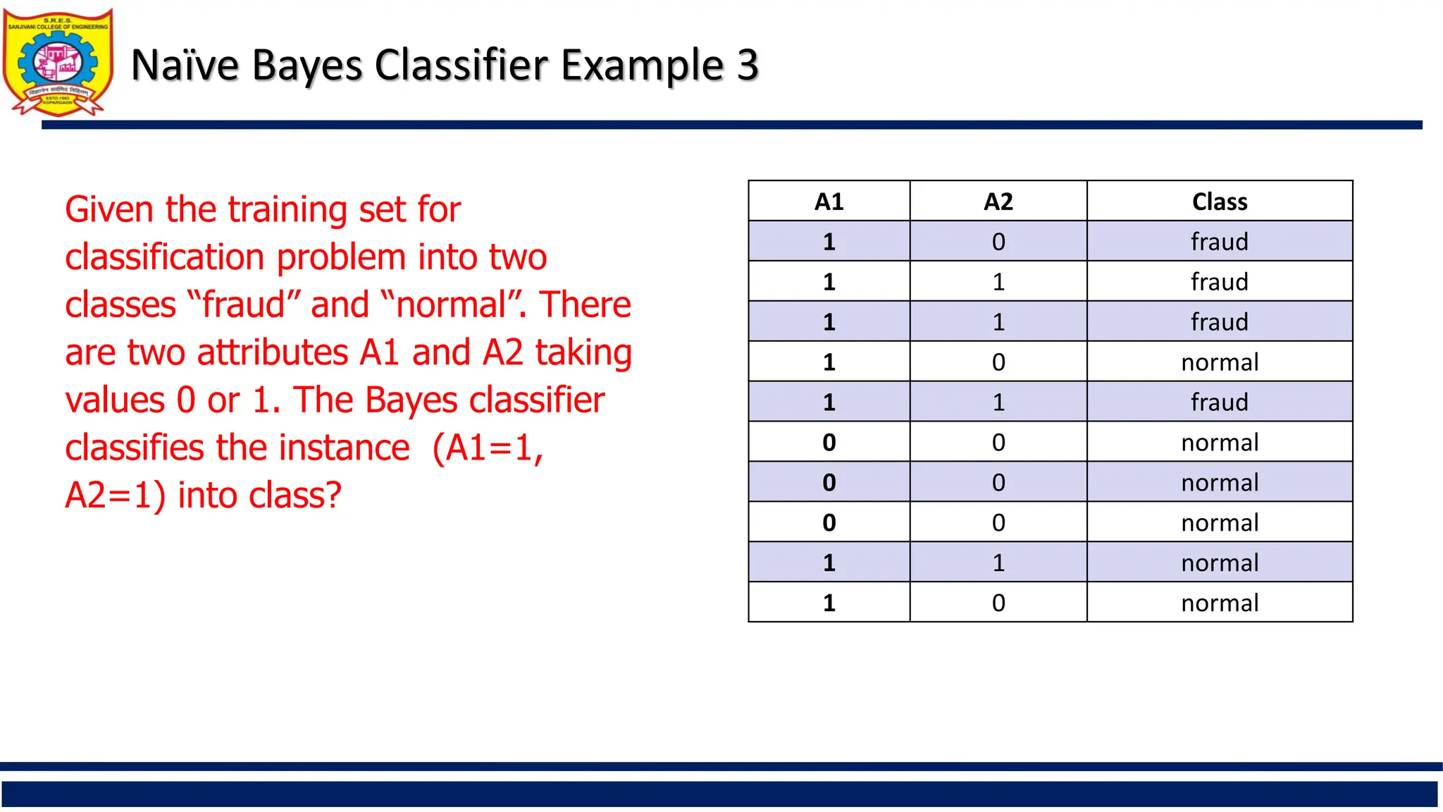
Given the training set for
classification problem into two
classes “fraud” and “normal”. There
are two attributes A1 and A2 taking
values 0 or 1. The Bayes classifier
classifies the instance (A1=1,
A2=1) into class?
A1 A2 Class
1 0 fraud
1 1 fraud
1 1 fraud
1 0 normal
1 1 fraud
0 0 normal
0 0 normal
0 0 normal
1 1 normal
1 0 normal
24.
Benefits of NaïveBayes Classifier
It is simple and easy to implement
It doesn’t require as much training data
It handles both continuous and discrete data
It is highly scalable with the number of predictors and data
points
It is fast and can be used to make real-time predictions
It is not sensitive to irrelevant features
25.
Limitations of NaïveBayes Classifier
Naive Bayes assumes that all predictors (or features) are
independent, rarely happening in real life. This limits the
applicability of this algorithm in real-world use cases.
This algorithm faces the ‘zero-frequency problem’ where it assigns
zero probability to a categorical variable whose category in the test
data set wasn’t available in the training dataset. It would be best if
you used a smoothing technique to overcome this issue.
Its estimations can be wrong in some cases, so you shouldn’t take
its probability outputs very seriously.
26.
Type of Distancesused in Machine Learning algorithm
Distance metric are used to represent distances between any two
data points.
There are many distance metrics.
1. Euclidean Distance
2. Manhattan Distance
3. Minkowski Distance
4. Hamming Distance
27.
Type of Distancesused in Machine Learning algorithm
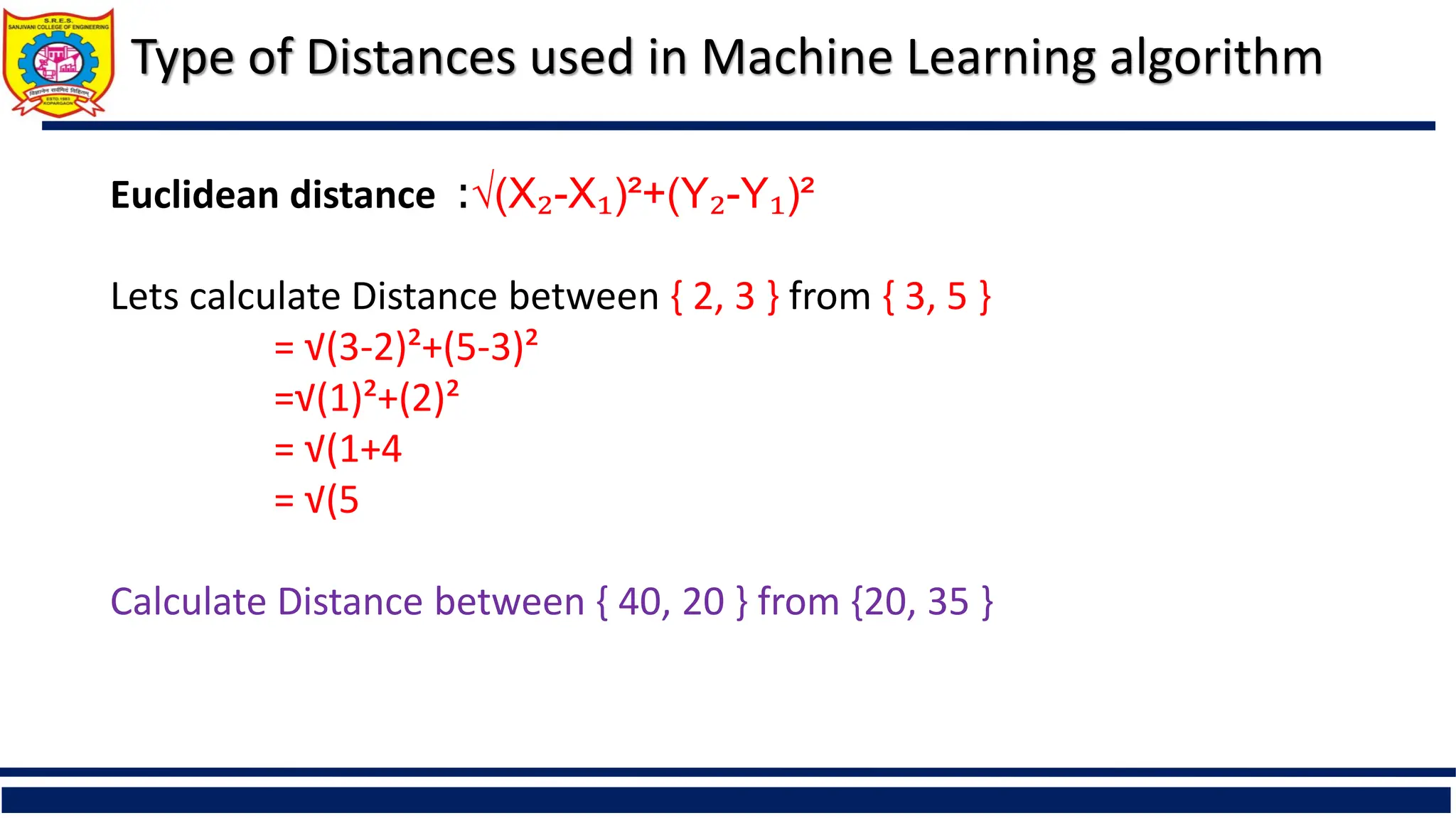
Euclidean distance :√(X₂-X₁)²+(Y₂-Y₁)²
Lets calculate Distance between { 2, 3 } from { 3, 5 }
= √(3-2)²+(5-3)²
=√(1)²+(2)²
= √(1+4
= √(5
Calculate Distance between { 40, 20 } from {20, 35 }
28.
Type of Distancesused in Machine Learning algorithm
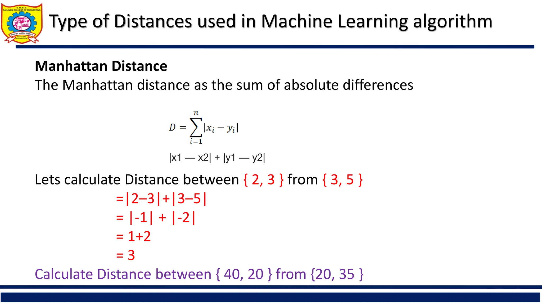
Manhattan Distance
The Manhattan distance as the sum of absolute differences
Lets calculate Distance between { 2, 3 } from { 3, 5 }
=|2–3|+|3–5|
= |-1| + |-2|
= 1+2
= 3
Calculate Distance between { 40, 20 } from {20, 35 }
|x1 — x2| + |y1 — y2|
29.
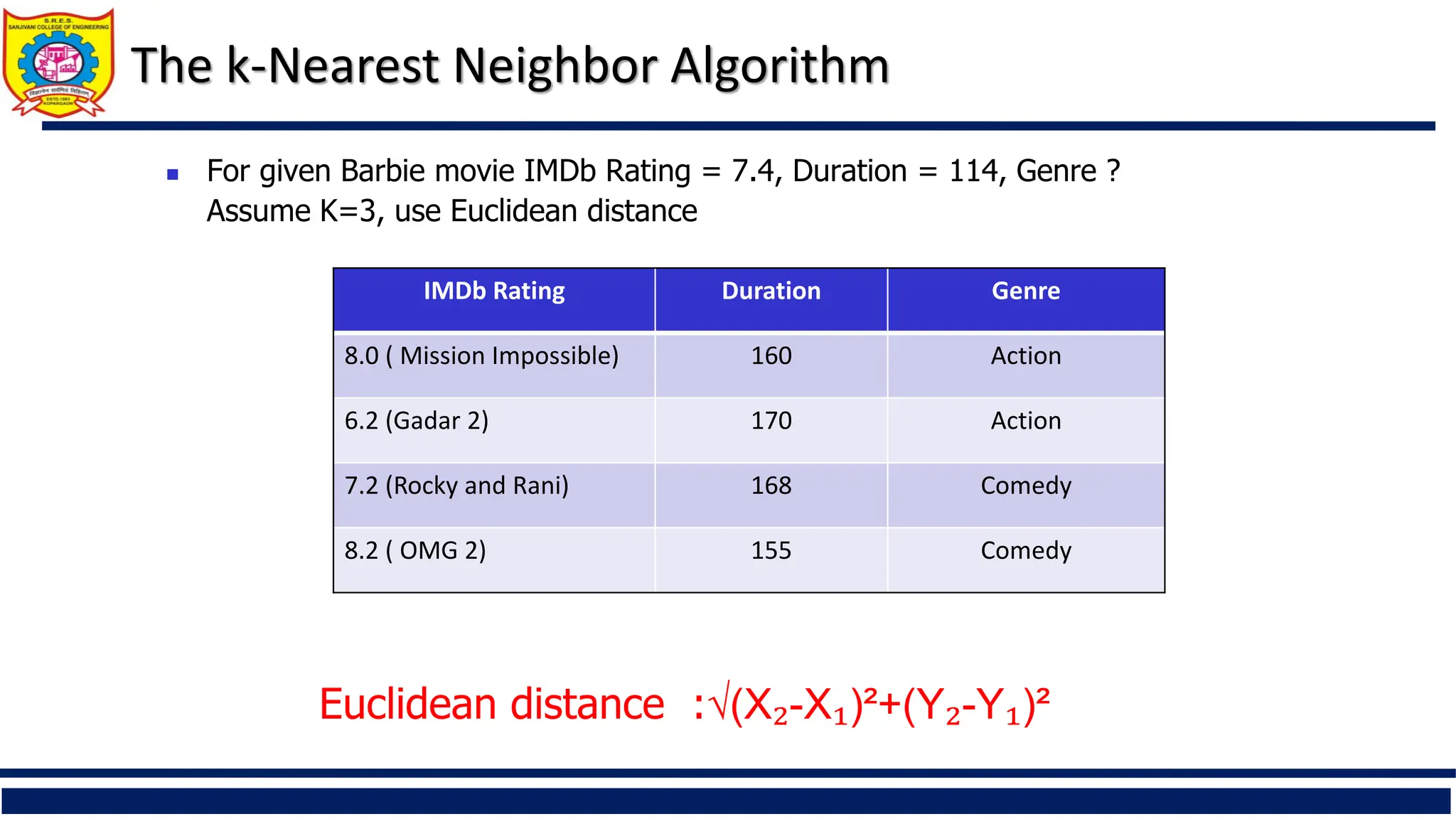
The k-Nearest NeighborAlgorithm
The k-nearest neighbors (KNN) algorithm is a non-parametric
Supervised learning classifier
Uses proximity to make classifications or predictions about the grouping of an
individual data point
Popular and simplest classification and regression classifiers used in machine
learning today
Mostly suited for Binary Classification
30.
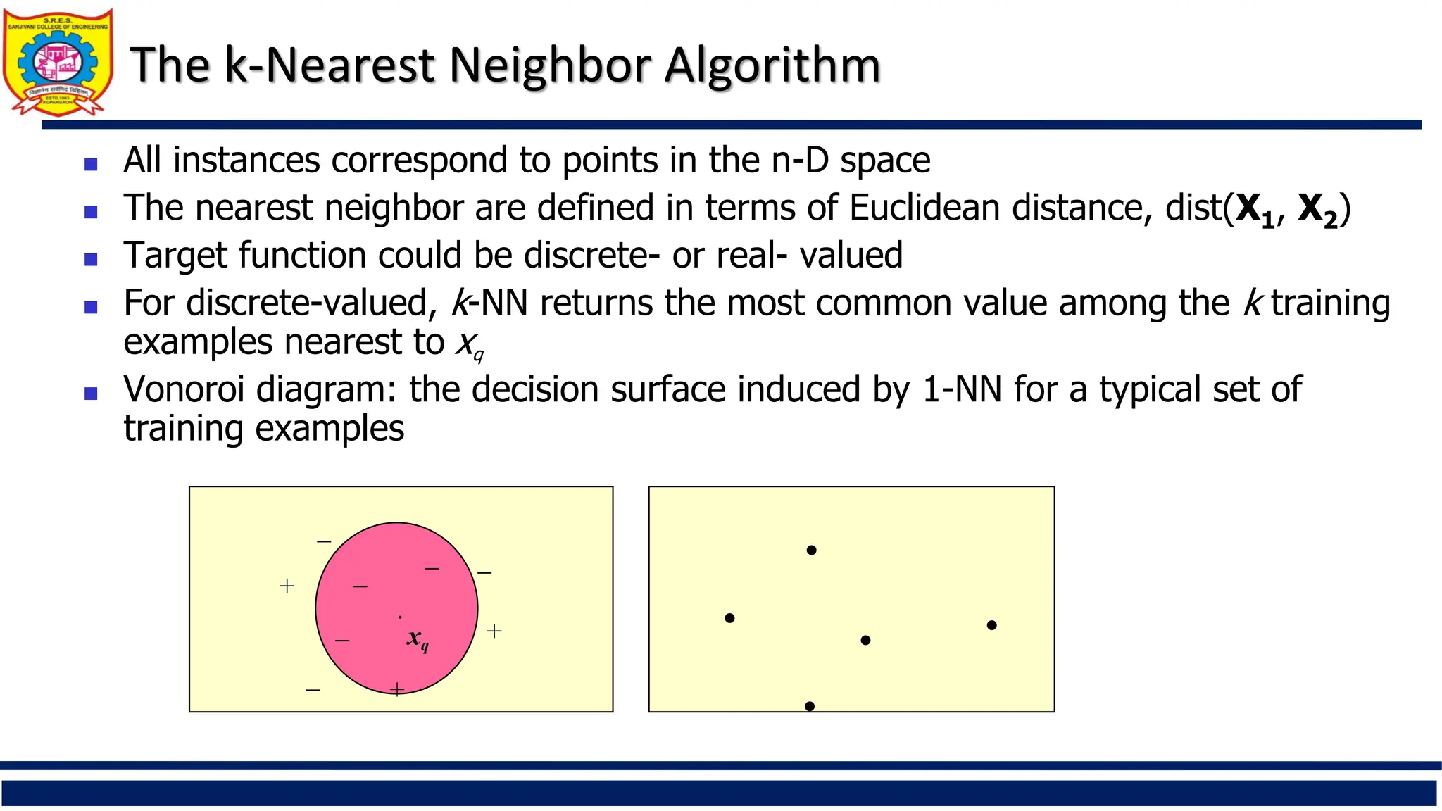
The k-Nearest NeighborAlgorithm
All instances correspond to points in the n-D space
The nearest neighbor are defined in terms of Euclidean distance, dist(X1, X2)
Target function could be discrete- or real- valued
For discrete-valued, k-NN returns the most common value among the k training
examples nearest to xq
Vonoroi diagram: the decision surface induced by 1-NN for a typical set of
training examples
.
_
_ xq
+
_ _
+
_
_
+
.
.
.
. .
31.
Step #1- Assign a value to K.
Step #2 - Calculate the distance between the new data entry and all
other existing data entries. Arrange them in ascending order.
Step #3 - Find the K nearest neighbors to the new entry based on the
calculated distances.
Step #4 - Assign the new data entry to the majority class in the
nearest neighbors.
The k-Nearest Neighbor Algorithm Steps
32.
Type of Distancesused in Machine Learning algorithm
Euclidean distance :√(X₂-X₁)²+(Y₂-Y₁)²
Lets calculate Distance between { 2, 3 } from { 3, 5 }
= √(3-2)²+(5-3)²
=√(1)²+(2)²
= √(1+4
= √(5
Calculate Distance between { 40, 20 } from {20, 35 }
33.
Type of Distancesused in Machine Learning algorithm
Manhattan Distance
The Manhattan distance as the sum of absolute differences
Lets calculate Distance between { 2, 3 } from { 3, 5 }
=|2–3|+|3–5|
= |-1| + |-2|
= 1+2
= 3
Calculate Distance between { 40, 20 } from {20, 35 }
|x1 — x2| + |y1 — y2|
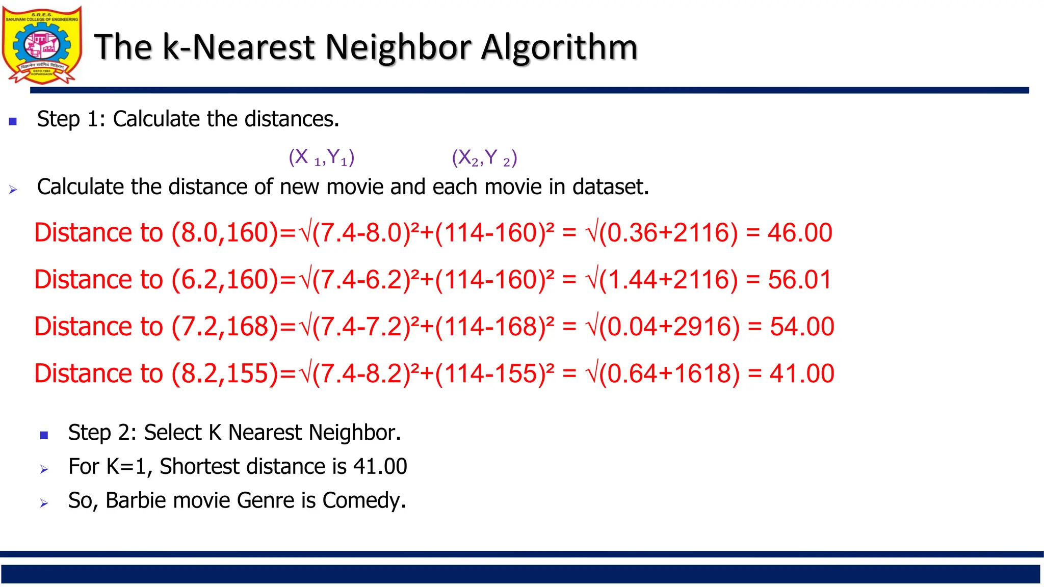
Step 1:Calculate the distances.
Calculate the distance of new movie and each movie in dataset.
Distance to (8.0,160)=√(7.4-8.0)²+(114-160)² = √(0.36+2116) = 46.00
Distance to (6.2,160)=√(7.4-6.2)²+(114-160)² = √(1.44+2116) = 56.01
Distance to (7.2,168)=√(7.4-7.2)²+(114-168)² = √(0.04+2916) = 54.00
Distance to (8.2,155)=√(7.4-8.2)²+(114-155)² = √(0.64+1618) = 41.00
The k-Nearest Neighbor Algorithm
(X ₁,Y₁) (X₂,Y ₂)
Step 2: Select K Nearest Neighbor.
For K=1, Shortest distance is 41.00
So, Barbie movie Genre is Comedy.
36.
The k-Nearest NeighborAlgorithm
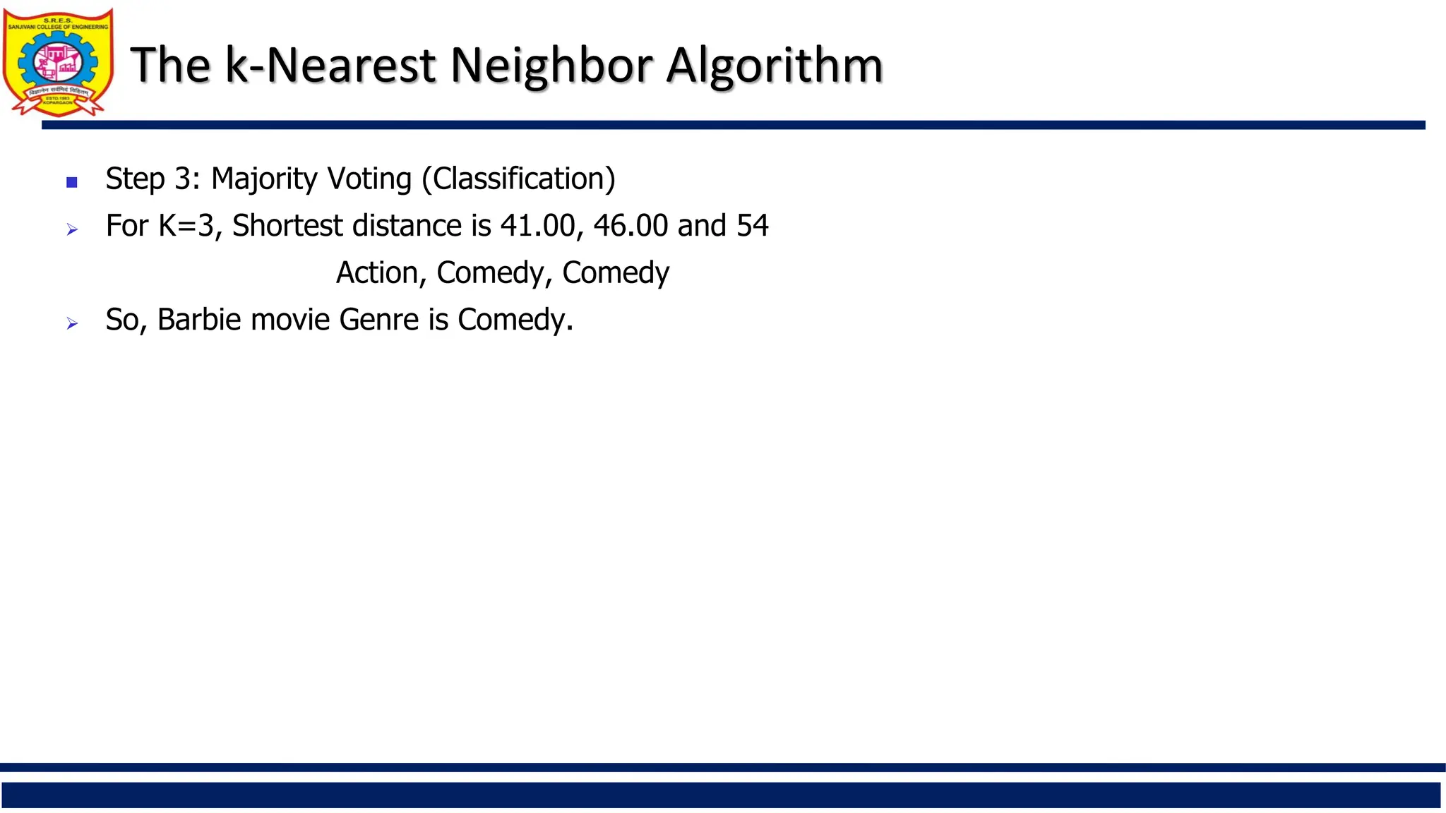
Step 3: Majority Voting (Classification)
For K=3, Shortest distance is 41.00, 46.00 and 54
Action, Comedy, Comedy
So, Barbie movie Genre is Comedy.
37.
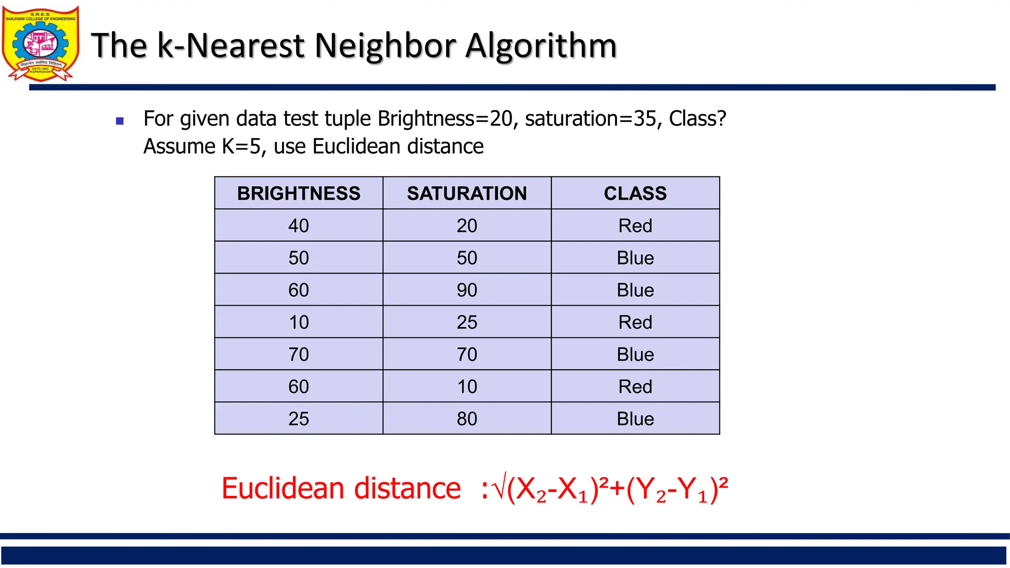
For givendata test tuple Brightness=20, saturation=35, Class?
Assume K=5, use Euclidean distance
BRIGHTNESS SATURATION CLASS
40 20 Red
50 50 Blue
60 90 Blue
10 25 Red
70 70 Blue
60 10 Red
25 80 Blue
Euclidean distance :√(X₂-X₁)²+(Y₂-Y₁)²
The k-Nearest Neighbor Algorithm
38.
DEPARTMENT OF COMPUTERENGINEERING, Sanjivani COE, Kopargaon 38
Reference
Han, Jiawei Kamber, Micheline Pei and Jian, “Data Mining: Concepts and
Techniques”,Elsevier Publishers, ISBN:9780123814791, 9780123814807.
https://onlinecourses.nptel.ac.in/noc24_cs22
https://medium.com/analytics-vidhya/type-of-distances-used-in-machine-
learning-algorithm-c873467140de
https://www.freecodecamp.org/news/k-nearest-neighbors-algorithm-
classifiers-and-model-example/