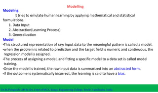
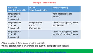
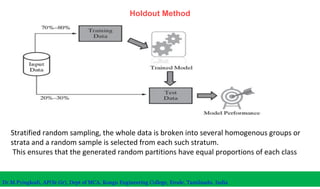
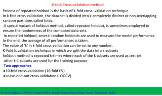
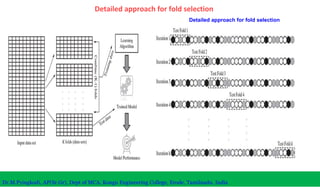
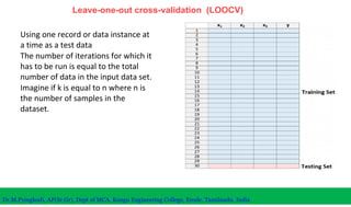
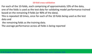
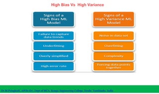
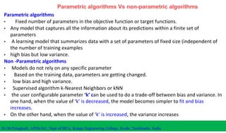
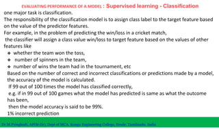
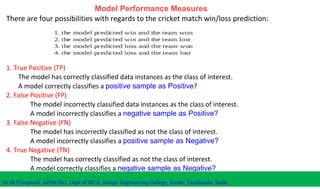
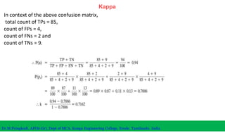
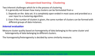
The document discusses machine learning concepts including modeling, evaluation, model selection, training models, and addressing issues like overfitting and underfitting. It explains that modeling tries to emulate human learning through mathematical and statistical formulations. Evaluation methods like holdout, k-fold cross-validation, and leave-one-out cross-validation are used to select models and train them on datasets while avoiding overfitting or underfitting issues. Parametric models have fixed parameters while non-parametric models are based on training data.

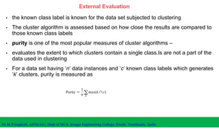
![Silhouette coefficient
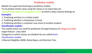
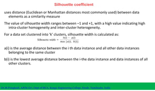
There are four clusters namely cluster 1, 2, 3, and 4.
data element ‘i’ in cluster 1, resembled by the asterisk. a(i) is the
average of the distances a ,
ai1,ai2,ai3, …ain
a of the different data elements from the ith data element in cluster 1
assuming there are n data elements in cluster 1.
Dr.M.Pyingkodi, AP(Sr.Gr), Dept of MCA, Kongu Engineering College, Erode, Tamilnadu, India
where n is the total number of elements in cluster 4. In the same way, we
can calculate the values of b (average) and b (average).
b (i) is the minimum of all these values.
b(i) = minimum [b (average), b (average), b (average)]](https://image.slidesharecdn.com/modellingandevaluationunit2june2322-220623063944-5c70ebed/85/Machine-Learning-Model-Evaluation-Methods-46-320.jpg)