SlideShare a Scribd company logo
1 of 7
Case Study # 3: Production/Cost & Perfect competition
(70pts total)
Fill in Answers below
Refer to case study for scenario and detailed instructions
Names of Team Members:_ Kayla Davenport_____
Part 1: Production and Cost (35pts)
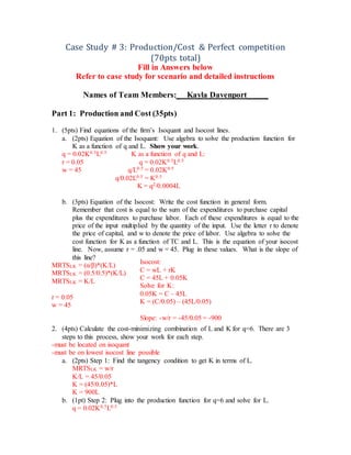
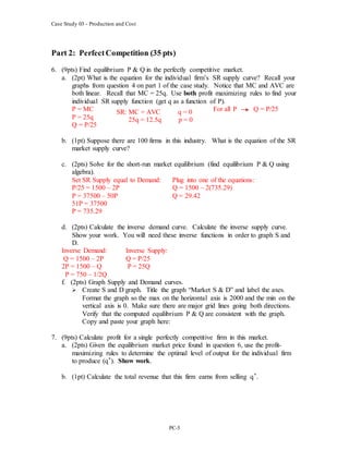
1. (5pts) Find equations of the firm’s Isoquant and Isocost lines.
a. (2pts) Equation of the Isoquant: Use algebra to solve the production function for
K as a function of q and L. Show your work.
q = 0.02K0.5L0.5 K as a function of q and L:
r = 0.05 q = 0.02K0.5L0.5
w = 45 q/L0.5 = 0.02K0.5
q/0.02L0.5 = K0.5
K = q2/0.0004L
b. (3pts) Equation of the Isocost: Write the cost function in general form.
Remember that cost is equal to the sum of the expenditures to purchase capital
plus the expenditures to purchase labor. Each of these expenditures is equal to the
price of the input multiplied by the quantity of the input. Use the letter r to denote
the price of capital, and w to denote the price of labor. Use algebra to solve the
cost function for K as a function of TC and L. This is the equation of your isocost
line. Now, assume r = .05 and w = 45. Plug in these values. What is the slope of
this line?
MRTSLK = (α/β)*(K/L)
MRTSLK = (0.5/0.5)*(K/L)
MRTSLK = K/L
r = 0.05
w = 45
2. (4pts) Calculate the cost-minimizing combination of L and K for q=6. There are 3
steps to this process, show your work for each step.
-must be located on isoquant
-must be on lowest isocost line possible
a. (2pts) Step 1: Find the tangency condition to get K in terms of L.
MRTSLK = w/r
K/L = 45/0.05
K = (45/0.05)*L
K = 900L
b. (1pt) Step 2: Plug into the production function for q=6 and solve for L.
q = 0.02K0.5L0.5
Isocost:
C = wL + rK
C = 45L + 0.05K
Solve for K:
0.05K = C – 45L
K = (C/0.05) – (45L/0.05)
Slope: -w/r = -45/0.05 = -900
Case Study 03 - Production and Cost
PC-2
6 = 0.02(900L)0.5*L0.5
6 = 0.02(30)L
6 = 0.6L
L = 10
c. (1pt) Step 3: Plug into the equation found in step 1 to find K.
K = 900L
K = 900(10)
K = 9,000
Total Cost: C = 45(10) + 0.05(9,000)
C = 900
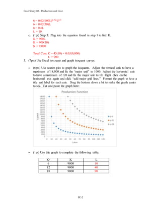
3. (7pts) Use Excel to create and graph isoquant curves:
 (6pts) Use scatter-plot to graph the isoquants. Adjust the vertical axis to have a
maximum of 18,000 and fix the “major unit” to 1000. Adjust the horizontal axis
to have a maximum of 120 and fix the major unit to 10. Right click on the
horizontal axis again and click “add major grid lines.” Format the graph to have a
title and label for each axis. Drag the bottom down a bit to make the graph easier
to see. Cut and paste the graph here:
 (1pt) Use this graph to complete the following table:
Q K L
6 9000 10
12 9000 40
18 9000 90
Case Study 03 - Production and Cost
PC-3
4. (15pts) Follow the steps below to find the short run cost curves associated with our
Cobb-Douglas production function when K is fixed at 9000 units. Assume r = .05
and w = 45.
a. (1.5pts) Calculate your SR production function (round any numbers to 4 decimal
places).
Q = 0.02(9000)0.5L0.5
Q = 1.8974*L0.5
b. (1.5pts) Calculate your FC.
FC = rK
FC = 450
c. (2pts) Derive the equation for your VC (as a function of q)
Q = 1.8974*L0.5
L0.5 = Q/1.8974
L = Q2/3.6
VC = wL
VC = 45*(Q2/3.6) = 12.5Q2
d. (1pt) Derive the equation for your TC (as a function of q)
TC = FC + VC
TC = 450 + 12.5Q2
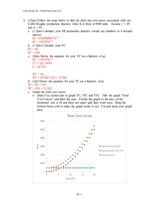
e. Graph the total cost curves:
 (4pts) Use scatter-plot to graph TC, TFC and TVC. Title the graph “Total
Cost Curves” and label the axes. Format the graph so the max on the
horizontal axis is 20 and there are major grid lines both ways. Drag the
bottom down a bit to make the graph easier to see. Cut and paste your graph
here:
Case Study 03 - Production and Cost
PC-4
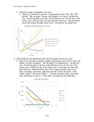
f. Graph the average and marginal cost curves:
 (5pts) Use scatter-plot to generate a second graph to show ATC, AFC, AVC
and MC. Title the graph “Average and Marginal Cost Curves” and label the
axes. Format the graph so the max on the horizontal axis is 20, the max on the
vertical axis is 500, and there are major grid lines both ways. Drag the bottom
down a bit to make the graph easier to see. Cut and paste your graph here:
5. (4pts) Graph the cost-minimizing point with the isoquant and isocost curves.
h. (4pts) Use scatter-plot to generate a graph of the isoquant and 3 isocost curves and
indicate the point of tangency. Title the graph “Cost Minimization” and label the
axes. Format the graph so the max on the horizontal axis is 35, the max on the
vertical axis is 25,000, the min on the vertical axis is 0, and there are major grid
lines both ways. Drag the bottom down a bit to make the graph easier to see.
Click on tangency point twice, right click and click “format data point.” Click
“marker options” and choose “built-in.” From the drop-down menu, choose the
circle and increase its size to 7. Click close. Cut and paste your graph here:
Case Study 03 - Production and Cost
PC-5
Part 2: PerfectCompetition (35 pts)
6. (9pts) Find equilibrium P & Q in the perfectly competitive market.
a. (2pt) What is the equation for the individual firm’s SR supply curve? Recall your
graphs from question 4 on part 1 of the case study. Notice that MC and AVC are
both linear. Recall that MC = 25q. Use both profit maximizing rules to find your
individual SR supply function (get q as a function of P).
P = MC For all P Q = P/25
P = 25q
Q = P/25
b. (1pt) Suppose there are 100 firms in this industry. What is the equation of the SR
market supply curve?
c. (2pts) Solve for the short-run market equilibrium (find equilibrium P & Q using
algebra).
Set SR Supply equal to Demand: Plug into one of the equations:
P/25 = 1500 – 2P Q = 1500 – 2(735.29)
P = 37500 – 50P Q = 29.42
51P = 37500
P = 735.29
d. (2pts) Calculate the inverse demand curve. Calculate the inverse supply curve.
Show your work. You will need these inverse functions in order to graph S and
D.
Inverse Demand: Inverse Supply:
Q = 1500 – 2P Q = P/25
2P = 1500 – Q P = 25Q
P = 750 – 1/2Q
f. (2pts) Graph Supply and Demand curves.
 Create S and D graph. Title the graph “Market S & D” and label the axes.
Format the graph so the max on the horizontal axis is 2000 and the min on the
vertical axis is 0. Make sure there are major grid lines going both directions.
Verify that the computed equilibrium P & Q are consistent with the graph.
Copy and paste your graph here:
7. (9pts) Calculate profit for a single perfectly competitive firm in this market.
a. (2pts) Given the equilibrium market price found in question 6, use the profit-
maximizing rules to determine the optimal level of output for the individual firm
to produce (q*). Show work.
b. (1pt) Calculate the total revenue that this firm earns from selling q*.
SR: MC = AVC q = 0
25q = 12.5q p = 0
Case Study 03 - Production and Cost
PC-6
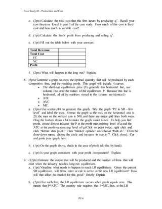
c. (2pts) Calculate the total cost that this firm incurs by producing q*. Recall your
cost functions found in part 1 of the case study. How much of this cost is fixed
cost and how much is variable cost?
d. (1pt) Calculate this firm’s profit from producing and selling q*.
e. (1pt) Fill out the table below with your answers:
Total Revenue
Total Cost
FC
VC
Profit
f. (2pts) What will happen in the long run? Explain.
8. (5pts) Generate a graph to show the optimal quantity that will be produced by each
competitive firm, and the resulting profit. This graph will include 4 curves:
 The short-run equilibrium price (To generate this horizontal line, use
column J to store the values of the equilibrium P. Because this line is
horizontal, all of the numbers stored in this column are identical.)
 ATC
 AVC
 MC.
a. (3pts) Use scatter-plot to generate this graph. Title the graph “PC in SR – firm
level” and label the axes. Format the graph so the max on the horizontal axis is
20, the max on the vertical axis is 500, and there are major grid lines both ways.
Drag the bottom down a bit to make the graph easier to see. To help you find
profit, create dots to indicate the P at the profit-maximizing level of q and the
ATC at the profit-maximizing level of q (Click on point twice, right click and
click “format data point.” Click “marker options” and choose “built-in.” From the
drop-down menu, choose the circle and increase its size to 7. Click close). Cut
and paste your graph here:
b. (1pt) On the graph above, shade in the area of profit (do this by hand).
c. (1pt) Is your graph consistent with your profit computation? Explain.
9. (12pts) Estimate the output that will be produced and the number of firms that will
exist when the industry reaches long-run equilibrium.
a. (1pt) Visualize what needs to happen to reach LR equilibrium. Given the current
SR equilibrium, will firms enter or exit to arrive at the new LR equilibrium? How
will that affect the market for this good? Briefly Explain.
b. (2pts) For each firm, the LR equilibrium occurs when profit equals zero. This
means that P=ATC. The quantity rule requires that P=MC, thus, at the LR
Case Study 03 - Production and Cost
PC-7
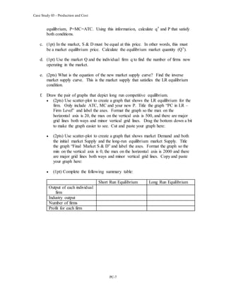
equilibrium, P=MC=ATC. Using this information, calculate q* and P that satisfy
both conditions.
c. (1pt) In the market, S & D must be equal at this price. In other words, this must
be a market equilibrium price. Calculate the equilibrium market quantity (Q*).
d. (1pt) Use the market Q and the individual firm q to find the number of firms now
operating in the market.
e. (2pts) What is the equation of the new market supply curve? Find the inverse
market supply curve. This is the market supply that satisfies the LR equilibrium
condition.
f. Draw the pair of graphs that depict long run competitive equilibrium.
 (2pts) Use scatter-plot to create a graph that shows the LR equilibrium for the
firm. Only include ATC, MC and your new P. Title the graph “PC in LR –
Firm Level” and label the axes. Format the graph so the max on the
horizontal axis is 20, the max on the vertical axis is 500, and there are major
grid lines both ways and minor vertical grid lines. Drag the bottom down a bit
to make the graph easier to see. Cut and paste your graph here:
 (2pts) Use scatter-plot to create a graph that shows market Demand and both
the initial market Supply and the long-run equilibrium market Supply. Title
the graph “Final Market S & D” and label the axes. Format the graph so the
min on the vertical axis is 0, the max on the horizontal axis is 2000 and there
are major grid lines both ways and minor vertical grid lines. Copy and paste
your graph here:
 (1pt) Complete the following summary table:
Short Run Equilibrium Long Run Equilibrium
Output of each individual
firm
Industry output
Number of firms
Profit for each firm

More Related Content

What's hot

What's hot (20)

Contract Costing
Contract CostingContract Costing
Contract Costing
 
Capital structure-theories
Capital structure-theoriesCapital structure-theories
Capital structure-theories
 
Pay back period ..chapter solution to problems...
Pay back period ..chapter solution to problems...Pay back period ..chapter solution to problems...
Pay back period ..chapter solution to problems...
 
Cost of capital
Cost of capitalCost of capital
Cost of capital
 
PORTFOLIO PERFORMANCE EVALUATION
PORTFOLIO PERFORMANCE EVALUATIONPORTFOLIO PERFORMANCE EVALUATION
PORTFOLIO PERFORMANCE EVALUATION
 
Forecasting
ForecastingForecasting
Forecasting
 
Payback period by harikrishnanan
Payback period by harikrishnananPayback period by harikrishnanan
Payback period by harikrishnanan
 
Elements of cost
Elements of costElements of cost
Elements of cost
 
Walter And Gordan theories
Walter And Gordan theoriesWalter And Gordan theories
Walter And Gordan theories
 
RISK ANALYSIS IN CAPITAL BUDGETING
RISK ANALYSIS IN CAPITAL BUDGETINGRISK ANALYSIS IN CAPITAL BUDGETING
RISK ANALYSIS IN CAPITAL BUDGETING
 
Value chain analysis
Value chain analysisValue chain analysis
Value chain analysis
 
Net Present Value - NPV
Net Present Value - NPVNet Present Value - NPV
Net Present Value - NPV
 
Project finance
Project financeProject finance
Project finance
 
WORKING CAPITAL MANAGEMENT
WORKING CAPITAL MANAGEMENTWORKING CAPITAL MANAGEMENT
WORKING CAPITAL MANAGEMENT
 
Gordon's model
Gordon's modelGordon's model
Gordon's model
 
Dividend decision theories
Dividend decision theoriesDividend decision theories
Dividend decision theories
 
Bond valuation
Bond valuationBond valuation
Bond valuation
 
compounding and discounting
compounding and discountingcompounding and discounting
compounding and discounting
 
Managerial Economics Production Analysis ppt by NDP
Managerial Economics Production Analysis ppt by NDPManagerial Economics Production Analysis ppt by NDP
Managerial Economics Production Analysis ppt by NDP
 
Marginal costing
Marginal costingMarginal costing
Marginal costing
 

Similar to Case Study 3 Production Cost Perfect Comp Answer Sheet - new

Exposure Interval Initial Risk Assessment (with exist.docx
Exposure Interval    Initial Risk Assessment (with exist.docxExposure Interval    Initial Risk Assessment (with exist.docx
Exposure Interval Initial Risk Assessment (with exist.docx
ssuser454af01
 
ECO 520 Case Study One Production and Cost Guidelines and Rubric.docx
ECO 520 Case Study One Production and Cost Guidelines and Rubric.docxECO 520 Case Study One Production and Cost Guidelines and Rubric.docx
ECO 520 Case Study One Production and Cost Guidelines and Rubric.docx
jack60216
 
ECO 520 Case Study One Production and Cost Guidelines and Rubri.docx
ECO 520 Case Study One Production and Cost Guidelines and Rubri.docxECO 520 Case Study One Production and Cost Guidelines and Rubri.docx
ECO 520 Case Study One Production and Cost Guidelines and Rubri.docx
jack60216
 
Article Critique Is genetic testing right for you and your f.docx
Article Critique Is genetic testing right for you and your f.docxArticle Critique Is genetic testing right for you and your f.docx
Article Critique Is genetic testing right for you and your f.docx
fredharris32
 
Class prodctn i
Class prodctn iClass prodctn i
Class prodctn i
mayankvns
 
Pre-Calculus Midterm Exam 1 Score ______ ____.docx
Pre-Calculus Midterm Exam  1  Score ______  ____.docxPre-Calculus Midterm Exam  1  Score ______  ____.docx
Pre-Calculus Midterm Exam 1 Score ______ ____.docx
ChantellPantoja184
 

Similar to Case Study 3 Production Cost Perfect Comp Answer Sheet - new (20)

Exposure Interval Initial Risk Assessment (with exist.docx
Exposure Interval    Initial Risk Assessment (with exist.docxExposure Interval    Initial Risk Assessment (with exist.docx
Exposure Interval Initial Risk Assessment (with exist.docx
 
ECO 520 Case Study One Production and Cost Guidelines and Rubric.docx
ECO 520 Case Study One Production and Cost Guidelines and Rubric.docxECO 520 Case Study One Production and Cost Guidelines and Rubric.docx
ECO 520 Case Study One Production and Cost Guidelines and Rubric.docx
 
ECO 520 Case Study One Production and Cost Guidelines and Rubri.docx
ECO 520 Case Study One Production and Cost Guidelines and Rubri.docxECO 520 Case Study One Production and Cost Guidelines and Rubri.docx
ECO 520 Case Study One Production and Cost Guidelines and Rubri.docx
 
Article Critique Is genetic testing right for you and your f.docx
Article Critique Is genetic testing right for you and your f.docxArticle Critique Is genetic testing right for you and your f.docx
Article Critique Is genetic testing right for you and your f.docx
 
Class prodctn i
Class prodctn iClass prodctn i
Class prodctn i
 
Fx570 ms 991ms_e
Fx570 ms 991ms_eFx570 ms 991ms_e
Fx570 ms 991ms_e
 
22424roduction Slides 33623-1.ppt
22424roduction Slides 33623-1.ppt22424roduction Slides 33623-1.ppt
22424roduction Slides 33623-1.ppt
 
Managerial_economics_paper.doc
Managerial_economics_paper.docManagerial_economics_paper.doc
Managerial_economics_paper.doc
 
Pre-Calculus Midterm Exam 1 Score ______ ____.docx
Pre-Calculus Midterm Exam  1  Score ______  ____.docxPre-Calculus Midterm Exam  1  Score ______  ____.docx
Pre-Calculus Midterm Exam 1 Score ______ ____.docx
 
Application of Mathematics in Business : F 107 - Group K
Application of Mathematics in Business : F 107 - Group KApplication of Mathematics in Business : F 107 - Group K
Application of Mathematics in Business : F 107 - Group K
 
Ch08
Ch08Ch08
Ch08
 
Chapter10 noha2012
Chapter10 noha2012Chapter10 noha2012
Chapter10 noha2012
 
Theory of production
Theory of productionTheory of production
Theory of production
 
Chapter 5 production process and cost
Chapter 5 production process and costChapter 5 production process and cost
Chapter 5 production process and cost
 
Using matlab simulink
Using matlab simulinkUsing matlab simulink
Using matlab simulink
 
Using matlab simulink
Using matlab simulinkUsing matlab simulink
Using matlab simulink
 
Microeconomics Production Cost
Microeconomics Production CostMicroeconomics Production Cost
Microeconomics Production Cost
 
Digital electronics k map comparators and their function
Digital electronics k map comparators and their functionDigital electronics k map comparators and their function
Digital electronics k map comparators and their function
 
lossless data compression and decompression using simple byte coding
lossless data compression and decompression using simple byte codinglossless data compression and decompression using simple byte coding
lossless data compression and decompression using simple byte coding
 
COST NOTES LECTURE ALL COST CURVES NUMERICALS EXAMPLES THEORY
COST NOTES LECTURE ALL COST CURVES NUMERICALS EXAMPLES THEORY COST NOTES LECTURE ALL COST CURVES NUMERICALS EXAMPLES THEORY
COST NOTES LECTURE ALL COST CURVES NUMERICALS EXAMPLES THEORY
 

Case Study 3 Production Cost Perfect Comp Answer Sheet - new

  • 1. Case Study # 3: Production/Cost & Perfect competition (70pts total) Fill in Answers below Refer to case study for scenario and detailed instructions Names of Team Members:_ Kayla Davenport_____ Part 1: Production and Cost (35pts) 1. (5pts) Find equations of the firm’s Isoquant and Isocost lines. a. (2pts) Equation of the Isoquant: Use algebra to solve the production function for K as a function of q and L. Show your work. q = 0.02K0.5L0.5 K as a function of q and L: r = 0.05 q = 0.02K0.5L0.5 w = 45 q/L0.5 = 0.02K0.5 q/0.02L0.5 = K0.5 K = q2/0.0004L b. (3pts) Equation of the Isocost: Write the cost function in general form. Remember that cost is equal to the sum of the expenditures to purchase capital plus the expenditures to purchase labor. Each of these expenditures is equal to the price of the input multiplied by the quantity of the input. Use the letter r to denote the price of capital, and w to denote the price of labor. Use algebra to solve the cost function for K as a function of TC and L. This is the equation of your isocost line. Now, assume r = .05 and w = 45. Plug in these values. What is the slope of this line? MRTSLK = (α/β)*(K/L) MRTSLK = (0.5/0.5)*(K/L) MRTSLK = K/L r = 0.05 w = 45 2. (4pts) Calculate the cost-minimizing combination of L and K for q=6. There are 3 steps to this process, show your work for each step. -must be located on isoquant -must be on lowest isocost line possible a. (2pts) Step 1: Find the tangency condition to get K in terms of L. MRTSLK = w/r K/L = 45/0.05 K = (45/0.05)*L K = 900L b. (1pt) Step 2: Plug into the production function for q=6 and solve for L. q = 0.02K0.5L0.5 Isocost: C = wL + rK C = 45L + 0.05K Solve for K: 0.05K = C – 45L K = (C/0.05) – (45L/0.05) Slope: -w/r = -45/0.05 = -900
  • 2. Case Study 03 - Production and Cost PC-2 6 = 0.02(900L)0.5*L0.5 6 = 0.02(30)L 6 = 0.6L L = 10 c. (1pt) Step 3: Plug into the equation found in step 1 to find K. K = 900L K = 900(10) K = 9,000 Total Cost: C = 45(10) + 0.05(9,000) C = 900 3. (7pts) Use Excel to create and graph isoquant curves:  (6pts) Use scatter-plot to graph the isoquants. Adjust the vertical axis to have a maximum of 18,000 and fix the “major unit” to 1000. Adjust the horizontal axis to have a maximum of 120 and fix the major unit to 10. Right click on the horizontal axis again and click “add major grid lines.” Format the graph to have a title and label for each axis. Drag the bottom down a bit to make the graph easier to see. Cut and paste the graph here:  (1pt) Use this graph to complete the following table: Q K L 6 9000 10 12 9000 40 18 9000 90
  • 3. Case Study 03 - Production and Cost PC-3 4. (15pts) Follow the steps below to find the short run cost curves associated with our Cobb-Douglas production function when K is fixed at 9000 units. Assume r = .05 and w = 45. a. (1.5pts) Calculate your SR production function (round any numbers to 4 decimal places). Q = 0.02(9000)0.5L0.5 Q = 1.8974*L0.5 b. (1.5pts) Calculate your FC. FC = rK FC = 450 c. (2pts) Derive the equation for your VC (as a function of q) Q = 1.8974*L0.5 L0.5 = Q/1.8974 L = Q2/3.6 VC = wL VC = 45*(Q2/3.6) = 12.5Q2 d. (1pt) Derive the equation for your TC (as a function of q) TC = FC + VC TC = 450 + 12.5Q2 e. Graph the total cost curves:  (4pts) Use scatter-plot to graph TC, TFC and TVC. Title the graph “Total Cost Curves” and label the axes. Format the graph so the max on the horizontal axis is 20 and there are major grid lines both ways. Drag the bottom down a bit to make the graph easier to see. Cut and paste your graph here:
  • 4. Case Study 03 - Production and Cost PC-4 f. Graph the average and marginal cost curves:  (5pts) Use scatter-plot to generate a second graph to show ATC, AFC, AVC and MC. Title the graph “Average and Marginal Cost Curves” and label the axes. Format the graph so the max on the horizontal axis is 20, the max on the vertical axis is 500, and there are major grid lines both ways. Drag the bottom down a bit to make the graph easier to see. Cut and paste your graph here: 5. (4pts) Graph the cost-minimizing point with the isoquant and isocost curves. h. (4pts) Use scatter-plot to generate a graph of the isoquant and 3 isocost curves and indicate the point of tangency. Title the graph “Cost Minimization” and label the axes. Format the graph so the max on the horizontal axis is 35, the max on the vertical axis is 25,000, the min on the vertical axis is 0, and there are major grid lines both ways. Drag the bottom down a bit to make the graph easier to see. Click on tangency point twice, right click and click “format data point.” Click “marker options” and choose “built-in.” From the drop-down menu, choose the circle and increase its size to 7. Click close. Cut and paste your graph here:
  • 5. Case Study 03 - Production and Cost PC-5 Part 2: PerfectCompetition (35 pts) 6. (9pts) Find equilibrium P & Q in the perfectly competitive market. a. (2pt) What is the equation for the individual firm’s SR supply curve? Recall your graphs from question 4 on part 1 of the case study. Notice that MC and AVC are both linear. Recall that MC = 25q. Use both profit maximizing rules to find your individual SR supply function (get q as a function of P). P = MC For all P Q = P/25 P = 25q Q = P/25 b. (1pt) Suppose there are 100 firms in this industry. What is the equation of the SR market supply curve? c. (2pts) Solve for the short-run market equilibrium (find equilibrium P & Q using algebra). Set SR Supply equal to Demand: Plug into one of the equations: P/25 = 1500 – 2P Q = 1500 – 2(735.29) P = 37500 – 50P Q = 29.42 51P = 37500 P = 735.29 d. (2pts) Calculate the inverse demand curve. Calculate the inverse supply curve. Show your work. You will need these inverse functions in order to graph S and D. Inverse Demand: Inverse Supply: Q = 1500 – 2P Q = P/25 2P = 1500 – Q P = 25Q P = 750 – 1/2Q f. (2pts) Graph Supply and Demand curves.  Create S and D graph. Title the graph “Market S & D” and label the axes. Format the graph so the max on the horizontal axis is 2000 and the min on the vertical axis is 0. Make sure there are major grid lines going both directions. Verify that the computed equilibrium P & Q are consistent with the graph. Copy and paste your graph here: 7. (9pts) Calculate profit for a single perfectly competitive firm in this market. a. (2pts) Given the equilibrium market price found in question 6, use the profit- maximizing rules to determine the optimal level of output for the individual firm to produce (q*). Show work. b. (1pt) Calculate the total revenue that this firm earns from selling q*. SR: MC = AVC q = 0 25q = 12.5q p = 0
  • 6. Case Study 03 - Production and Cost PC-6 c. (2pts) Calculate the total cost that this firm incurs by producing q*. Recall your cost functions found in part 1 of the case study. How much of this cost is fixed cost and how much is variable cost? d. (1pt) Calculate this firm’s profit from producing and selling q*. e. (1pt) Fill out the table below with your answers: Total Revenue Total Cost FC VC Profit f. (2pts) What will happen in the long run? Explain. 8. (5pts) Generate a graph to show the optimal quantity that will be produced by each competitive firm, and the resulting profit. This graph will include 4 curves:  The short-run equilibrium price (To generate this horizontal line, use column J to store the values of the equilibrium P. Because this line is horizontal, all of the numbers stored in this column are identical.)  ATC  AVC  MC. a. (3pts) Use scatter-plot to generate this graph. Title the graph “PC in SR – firm level” and label the axes. Format the graph so the max on the horizontal axis is 20, the max on the vertical axis is 500, and there are major grid lines both ways. Drag the bottom down a bit to make the graph easier to see. To help you find profit, create dots to indicate the P at the profit-maximizing level of q and the ATC at the profit-maximizing level of q (Click on point twice, right click and click “format data point.” Click “marker options” and choose “built-in.” From the drop-down menu, choose the circle and increase its size to 7. Click close). Cut and paste your graph here: b. (1pt) On the graph above, shade in the area of profit (do this by hand). c. (1pt) Is your graph consistent with your profit computation? Explain. 9. (12pts) Estimate the output that will be produced and the number of firms that will exist when the industry reaches long-run equilibrium. a. (1pt) Visualize what needs to happen to reach LR equilibrium. Given the current SR equilibrium, will firms enter or exit to arrive at the new LR equilibrium? How will that affect the market for this good? Briefly Explain. b. (2pts) For each firm, the LR equilibrium occurs when profit equals zero. This means that P=ATC. The quantity rule requires that P=MC, thus, at the LR
  • 7. Case Study 03 - Production and Cost PC-7 equilibrium, P=MC=ATC. Using this information, calculate q* and P that satisfy both conditions. c. (1pt) In the market, S & D must be equal at this price. In other words, this must be a market equilibrium price. Calculate the equilibrium market quantity (Q*). d. (1pt) Use the market Q and the individual firm q to find the number of firms now operating in the market. e. (2pts) What is the equation of the new market supply curve? Find the inverse market supply curve. This is the market supply that satisfies the LR equilibrium condition. f. Draw the pair of graphs that depict long run competitive equilibrium.  (2pts) Use scatter-plot to create a graph that shows the LR equilibrium for the firm. Only include ATC, MC and your new P. Title the graph “PC in LR – Firm Level” and label the axes. Format the graph so the max on the horizontal axis is 20, the max on the vertical axis is 500, and there are major grid lines both ways and minor vertical grid lines. Drag the bottom down a bit to make the graph easier to see. Cut and paste your graph here:  (2pts) Use scatter-plot to create a graph that shows market Demand and both the initial market Supply and the long-run equilibrium market Supply. Title the graph “Final Market S & D” and label the axes. Format the graph so the min on the vertical axis is 0, the max on the horizontal axis is 2000 and there are major grid lines both ways and minor vertical grid lines. Copy and paste your graph here:  (1pt) Complete the following summary table: Short Run Equilibrium Long Run Equilibrium Output of each individual firm Industry output Number of firms Profit for each firm