Download as PDF, PPTX


![CSCS in ECL
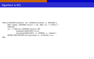
CSCS2(DATASET(Elem) YY, REAL lambda3, REAL tol2=0.00001,
UNSIGNED maxIter2=100) := FUNCTION
nobs := MAX(YY,x);
pvars := MAX(YY,y);
S:= Mat.Scale(Mat.Mul(Mat.Trans(YY),YY),(1/nobs));
S1 := DISTRIBUTE(NORMALIZE(S, (pvars DIV 2),
TRANSFORM(DistElem, SELF.nid:=COUNTER, SELF:=LEFT)), nid);
L:= Identity(pvars);
LL:= DISTRIBUTE(L,nid);
L11 := PROJECT(CHOOSEN(S1(x=1 AND y=1 AND nid=1),1),
TRANSFORM(DistElem, SELF.x := 1, SELF.y := 1,
SELF.value:=1/LEFT.value, SELF.nid := 1, SELF:=[]));
newL := LL(x <> 1) + L11;
newLL := LOOP(newL,COUNTER<pvars,OuterOuterBody(ROWS(LEFT), S1,
COUNTER, lambda3, maxIter2, tol2));
RETURN newLL;
END;
22 / 22](https://image.slidesharecdn.com/008rahmankhareuf-161020203416/85/Understanding-High-dimensional-Networks-for-Continuous-Variables-Using-ECL-23-320.jpg)

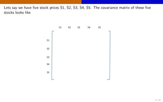
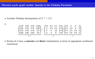
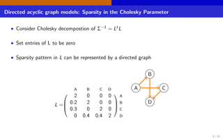
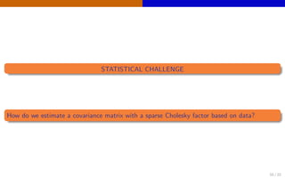
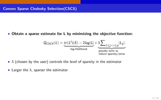
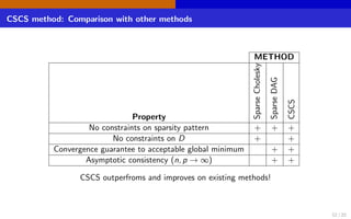
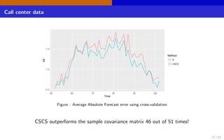
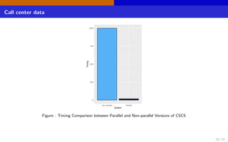
The document discusses high-dimensional networks for continuous variables, focusing on the challenges of estimating covariance matrices when the number of variables exceeds the sample size. It introduces a new method called Convex Sparse Cholesky Selection (CSCS) to effectively estimate sparse covariance matrices, demonstrating its superiority through a case study on call center data. The method achieves improved forecasting accuracy compared to traditional sample covariance techniques.


![7.__Developing_a_Research_Proposal[1].pptx](https://cdn.slidesharecdn.com/ss_thumbnails/7-260131073037-df92dd7d-thumbnail.jpg?width=640&height=640&fit=bounds)


![Hacking-Uncovered-How-People-Get-Hacked-and-How-to-Stay-Safe[1].pptx](https://cdn.slidesharecdn.com/ss_thumbnails/hacking-uncovered-how-people-get-hacked-and-how-to-stay-safe1-260130170011-4883a9c7-thumbnail.jpg?width=640&height=640&fit=bounds)


