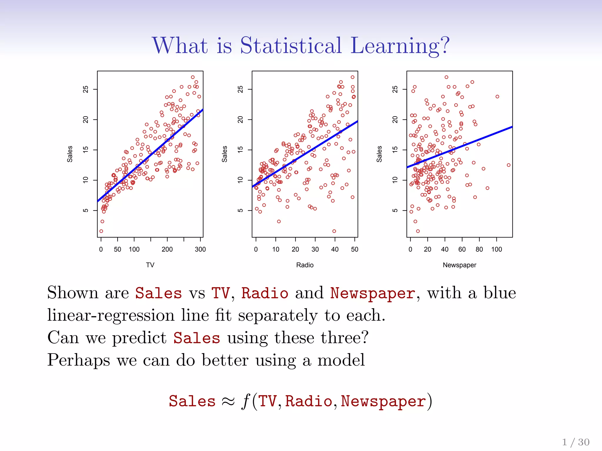
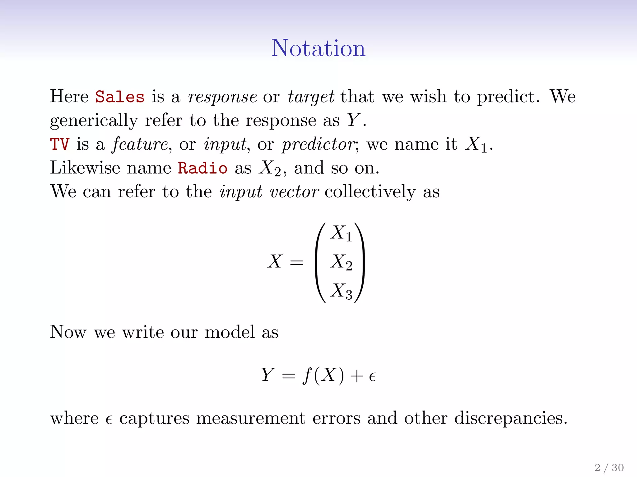
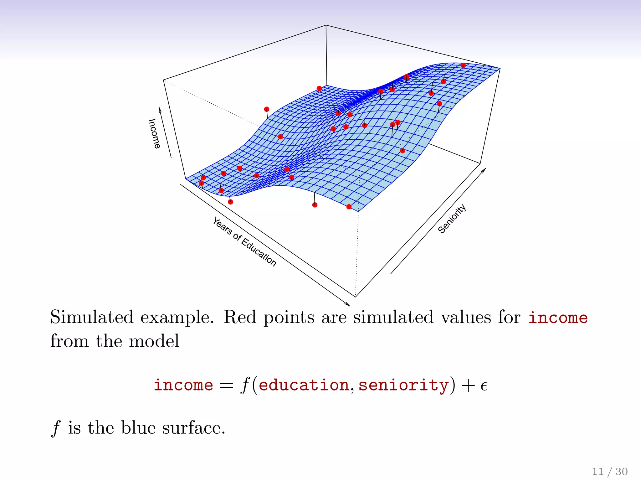
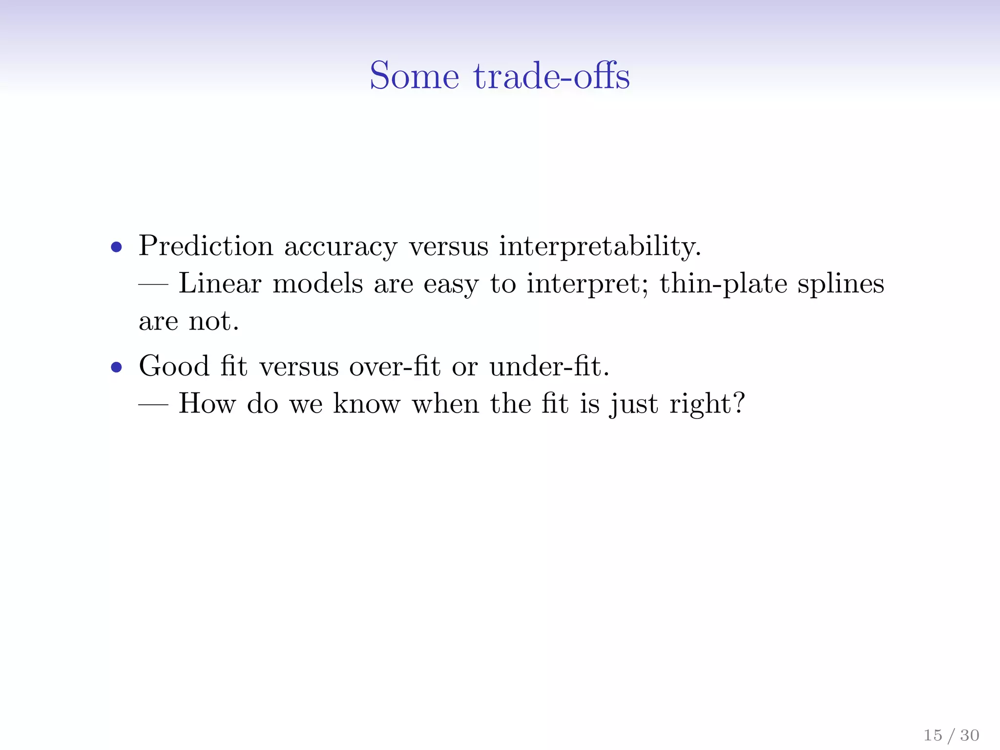
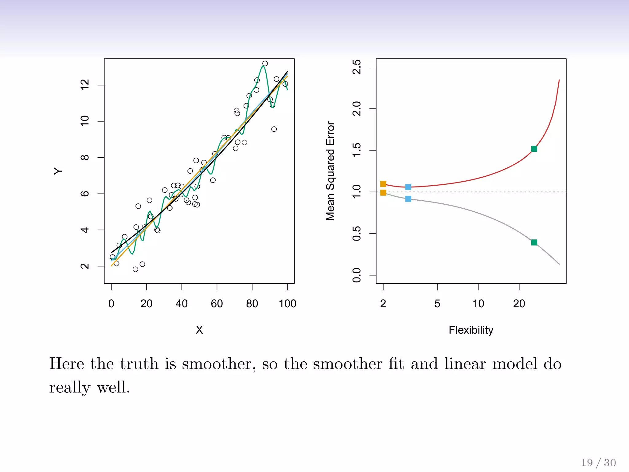
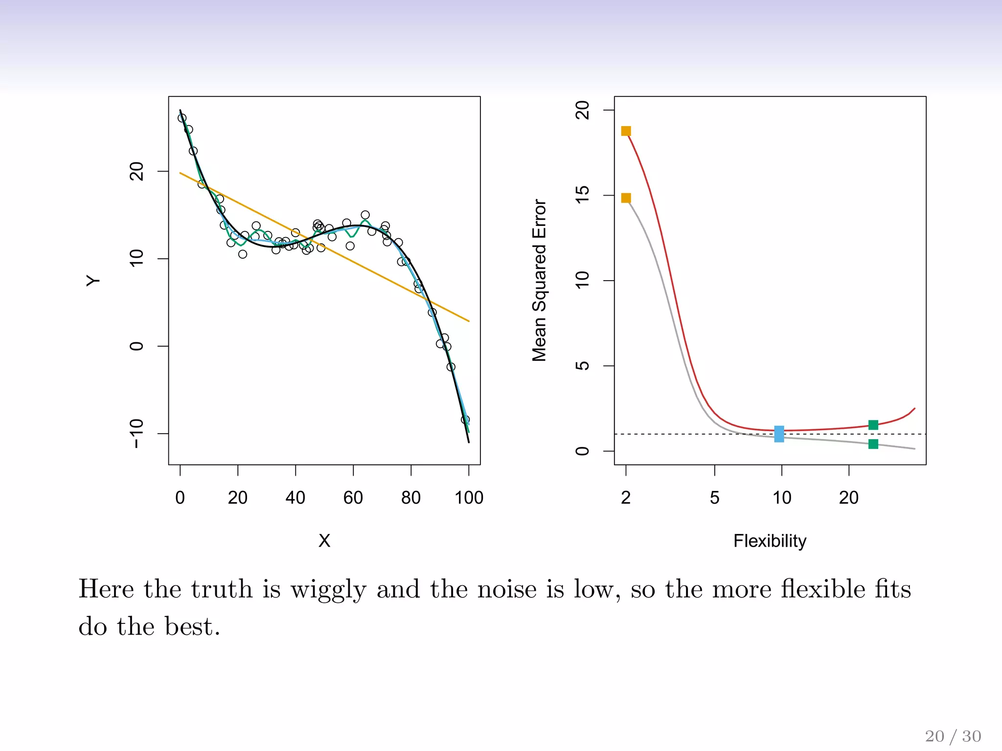
Statistical learning is a method for using variables like TV, radio and newspaper advertising spending (features) to predict sales (response). It builds a statistical model, Sales = f(TV, radio, newspaper), to understand the relationship between the features and response. This allows one to make sales predictions based on advertising spending and determine which features have the most influence on sales.
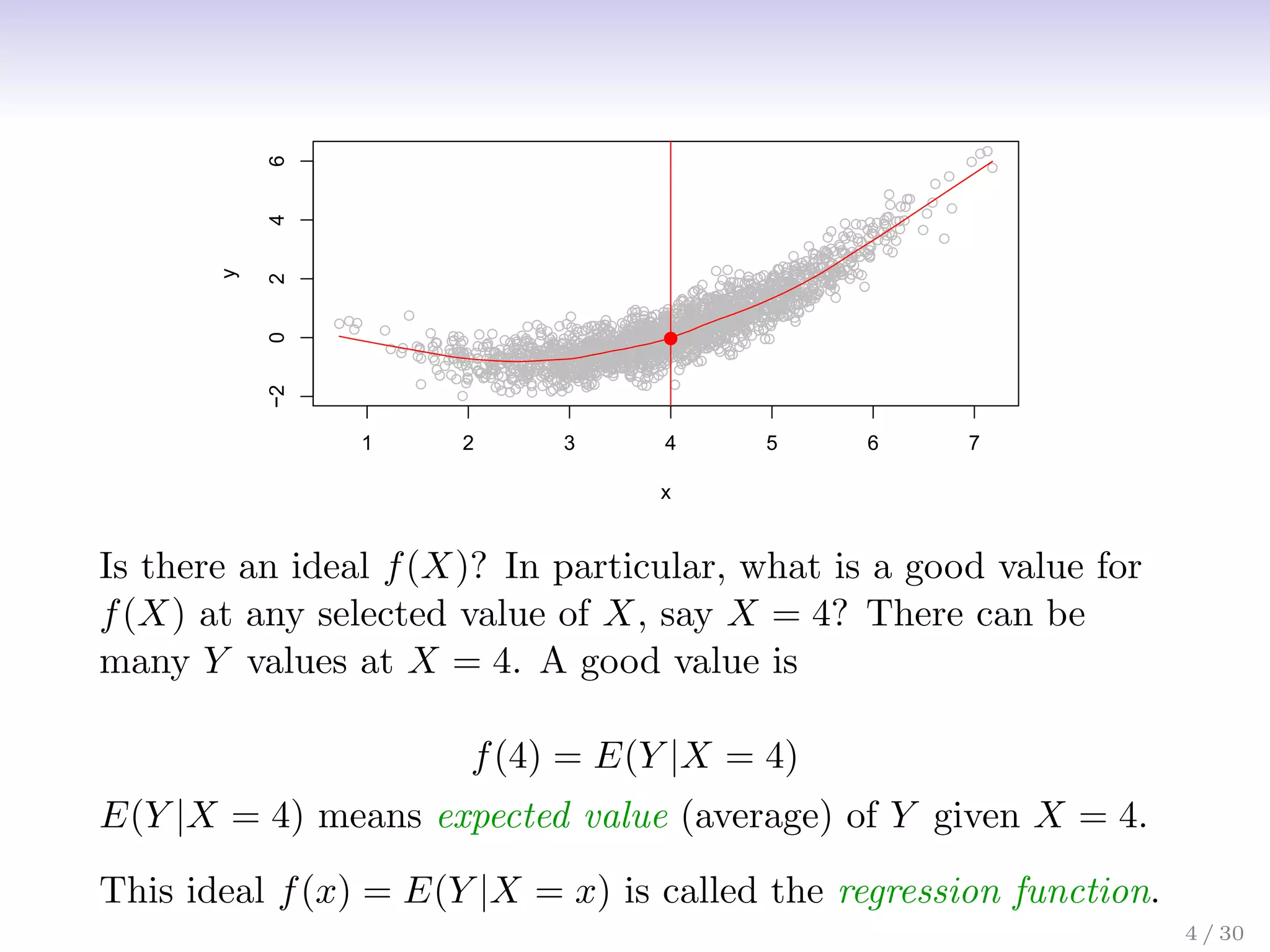
![The regression function f(x)
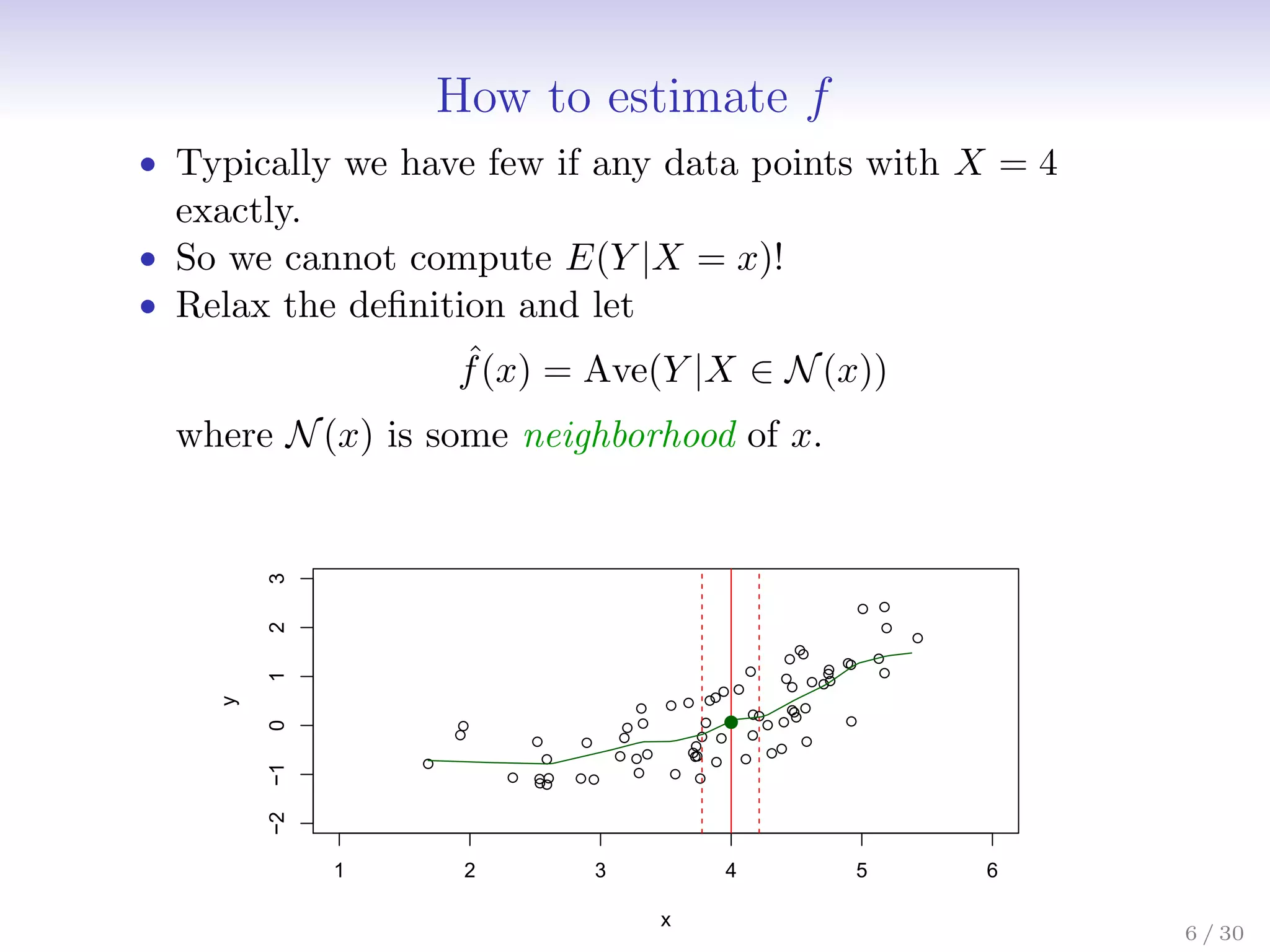
• Is also defined for vector X; e.g.
f(x) = f(x1, x2, x3) = E(Y |X1 = x1, X2 = x2, X3 = x3)
• Is the ideal or optimal predictor of Y with regard to
mean-squared prediction error: f(x) = E(Y |X = x) is the
function that minimizes E[(Y − g(X))2|X = x] over all
functions g at all points X = x.
5 / 30](https://image.slidesharecdn.com/ch2statisticallearning-230117050556-1e15522a/75/Ch2_Statistical_Learning-pdf-6-2048.jpg)
![The regression function f(x)
• Is also defined for vector X; e.g.
f(x) = f(x1, x2, x3) = E(Y |X1 = x1, X2 = x2, X3 = x3)
• Is the ideal or optimal predictor of Y with regard to
mean-squared prediction error: f(x) = E(Y |X = x) is the
function that minimizes E[(Y − g(X))2|X = x] over all
functions g at all points X = x.
• = Y − f(x) is the irreducible error — i.e. even if we knew
f(x), we would still make errors in prediction, since at each
X = x there is typically a distribution of possible Y values.
5 / 30](https://image.slidesharecdn.com/ch2statisticallearning-230117050556-1e15522a/75/Ch2_Statistical_Learning-pdf-7-2048.jpg)
![The regression function f(x)
• Is also defined for vector X; e.g.
f(x) = f(x1, x2, x3) = E(Y |X1 = x1, X2 = x2, X3 = x3)
• Is the ideal or optimal predictor of Y with regard to
mean-squared prediction error: f(x) = E(Y |X = x) is the
function that minimizes E[(Y − g(X))2|X = x] over all
functions g at all points X = x.
• = Y − f(x) is the irreducible error — i.e. even if we knew
f(x), we would still make errors in prediction, since at each
X = x there is typically a distribution of possible Y values.
• For any estimate ˆ
f(x) of f(x), we have
E[(Y − ˆ
f(X))2
|X = x] = [f(x) − ˆ
f(x)]2
| {z }
Reducible
+ Var()
| {z }
Irreducible
5 / 30](https://image.slidesharecdn.com/ch2statisticallearning-230117050556-1e15522a/75/Ch2_Statistical_Learning-pdf-8-2048.jpg)
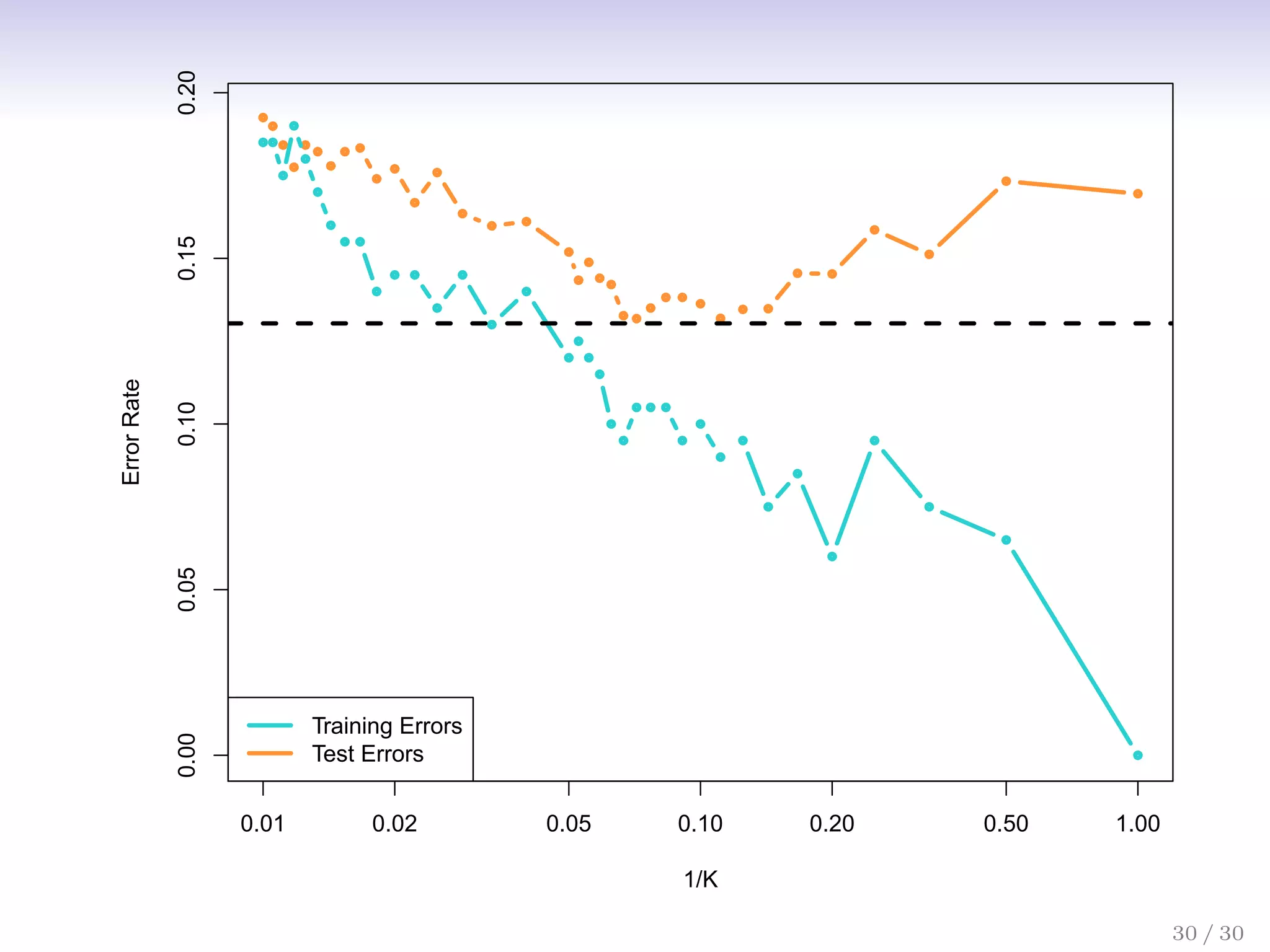
![Assessing Model Accuracy
Suppose we fit a model ˆ
f(x) to some training data
Tr = {xi, yi}N
1 , and we wish to see how well it performs.
• We could compute the average squared prediction error
over Tr:
MSETr = Avei∈Tr[yi − ˆ
f(xi)]2
This may be biased toward more overfit models.
• Instead we should, if possible, compute it using fresh test
data Te = {xi, yi}M
1 :
MSETe = Avei∈Te[yi − ˆ
f(xi)]2
17 / 30](https://image.slidesharecdn.com/ch2statisticallearning-230117050556-1e15522a/75/Ch2_Statistical_Learning-pdf-23-2048.jpg)
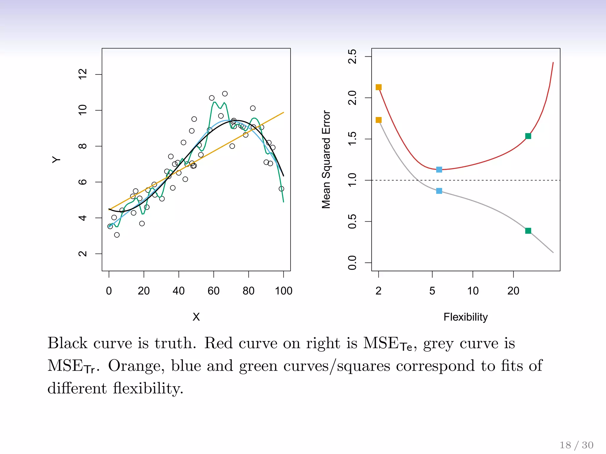
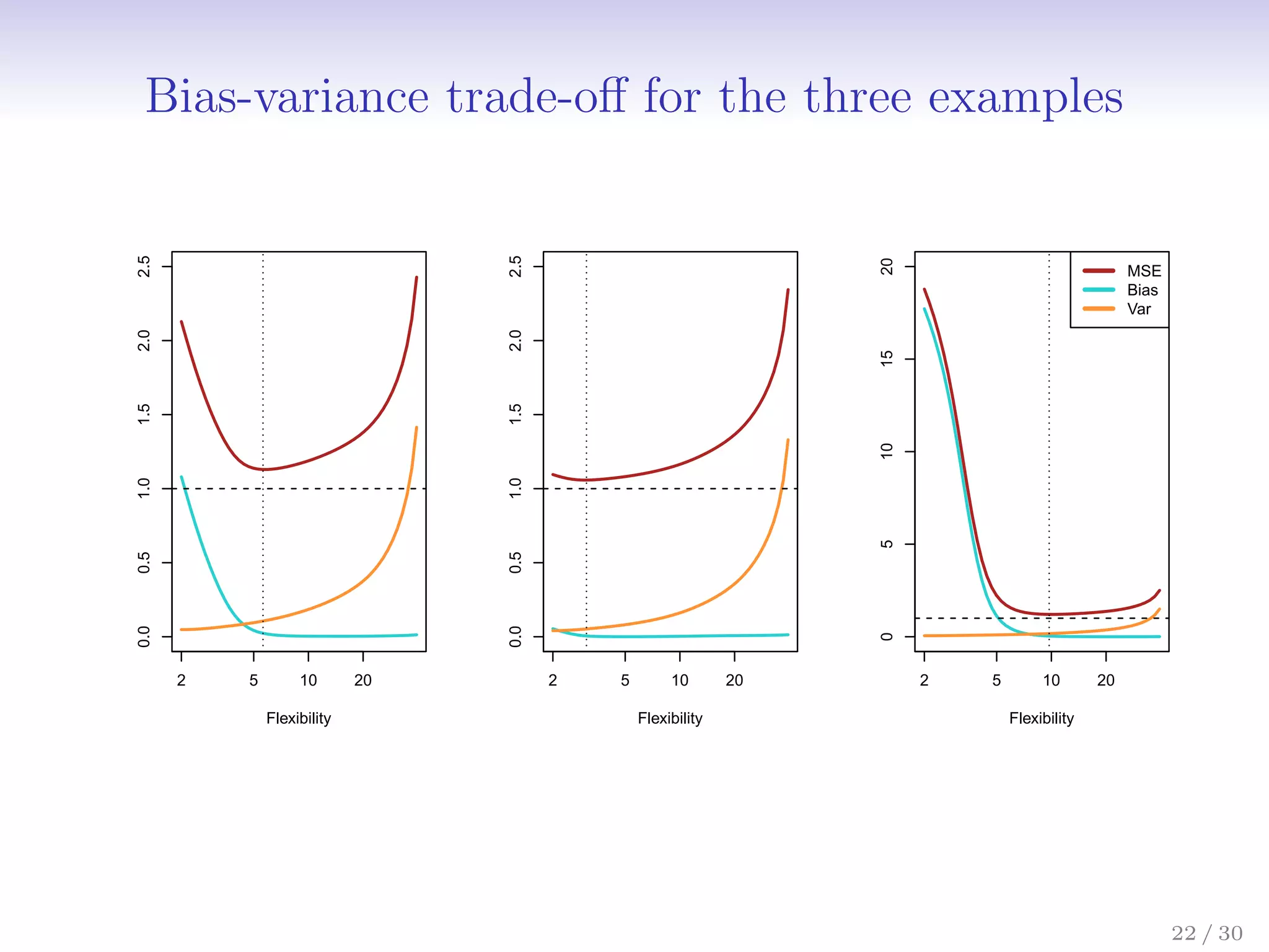
![Bias-Variance Trade-off
Suppose we have fit a model ˆ
f(x) to some training data Tr, and
let (x0, y0) be a test observation drawn from the population. If
the true model is Y = f(X) + (with f(x) = E(Y |X = x)),
then
E
y0 − ˆ
f(x0)
2
= Var( ˆ
f(x0)) + [Bias( ˆ
f(x0))]2
+ Var().
The expectation averages over the variability of y0 as well as
the variability in Tr. Note that Bias( ˆ
f(x0))] = E[ ˆ
f(x0)] − f(x0).
Typically as the flexibility of ˆ
f increases, its variance increases,
and its bias decreases. So choosing the flexibility based on
average test error amounts to a bias-variance trade-off.
21 / 30](https://image.slidesharecdn.com/ch2statisticallearning-230117050556-1e15522a/75/Ch2_Statistical_Learning-pdf-27-2048.jpg)
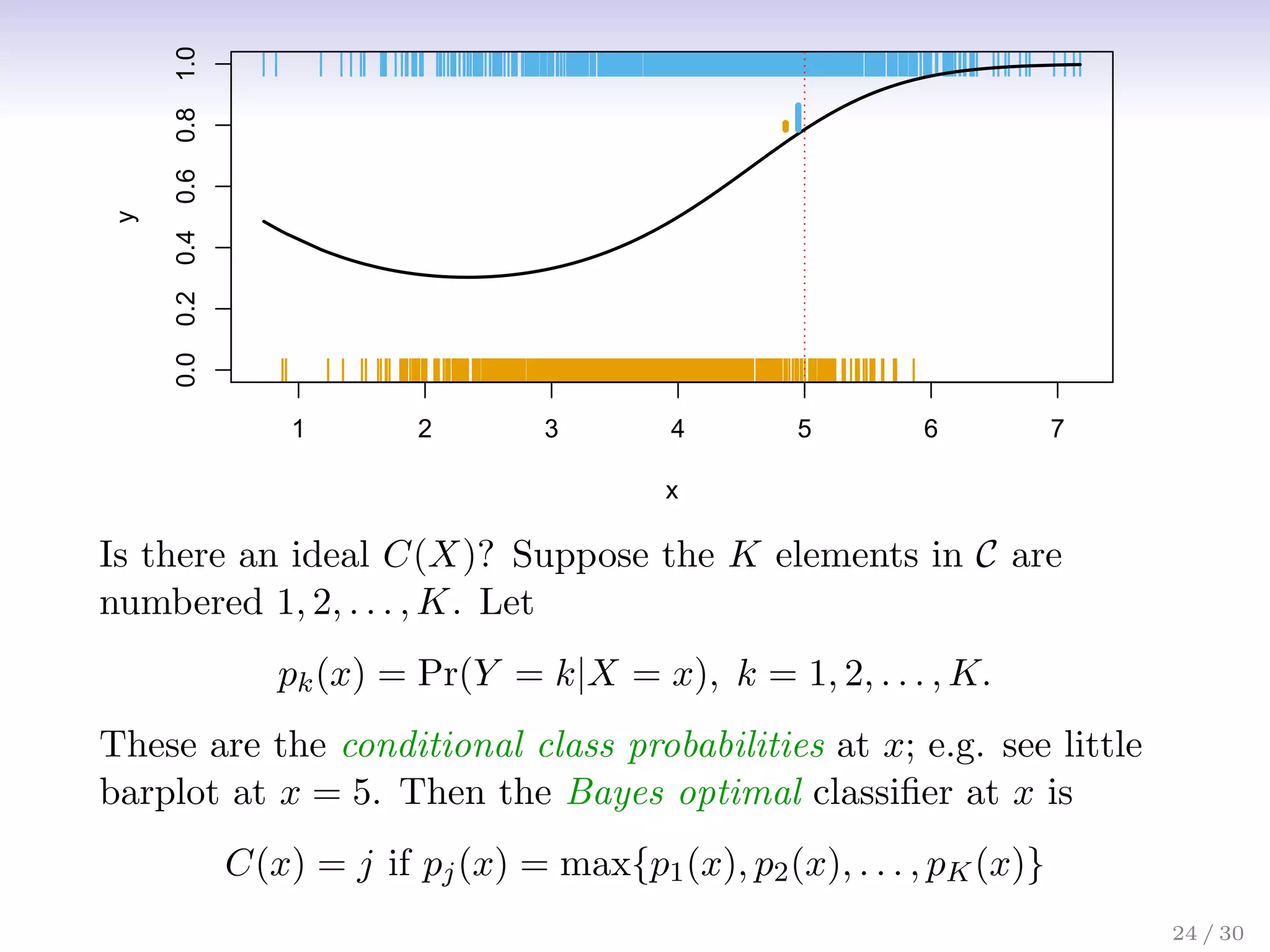
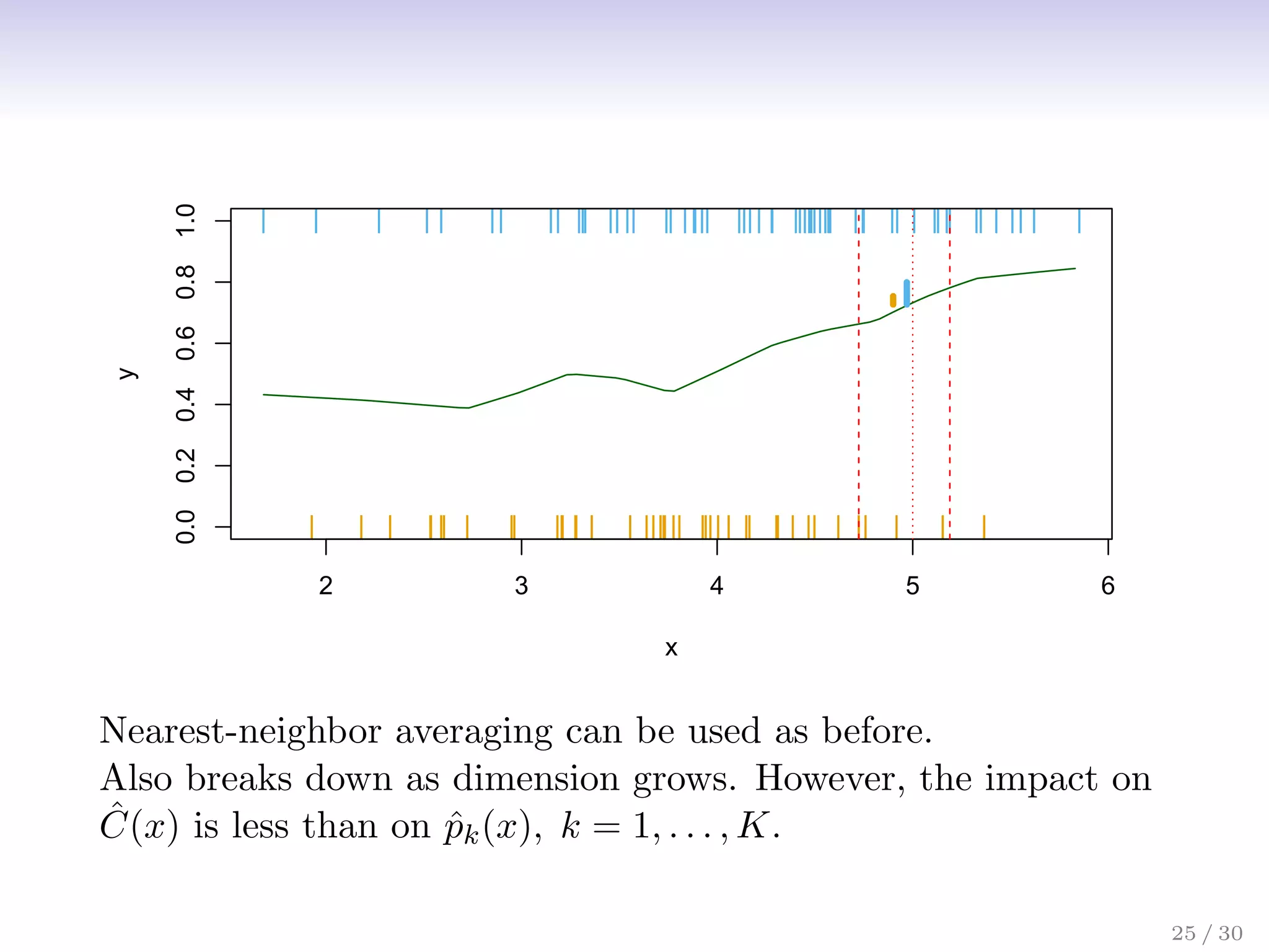
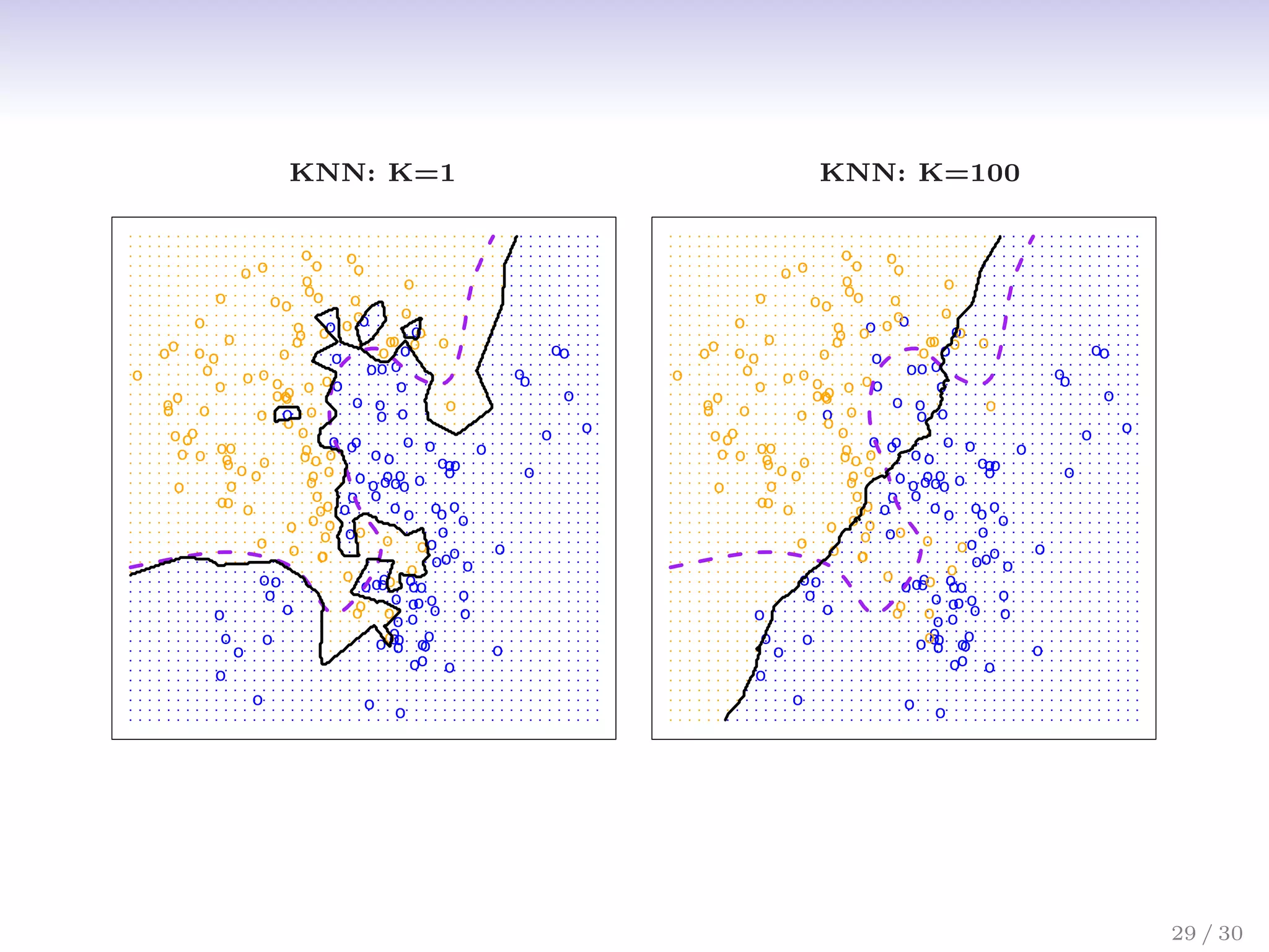
![Classification: some details
• Typically we measure the performance of Ĉ(x) using the
misclassification error rate:
ErrTe = Avei∈TeI[yi 6= Ĉ(xi)]
• The Bayes classifier (using the true pk(x)) has smallest
error (in the population).
26 / 30](https://image.slidesharecdn.com/ch2statisticallearning-230117050556-1e15522a/75/Ch2_Statistical_Learning-pdf-32-2048.jpg)
![Classification: some details
• Typically we measure the performance of Ĉ(x) using the
misclassification error rate:
ErrTe = Avei∈TeI[yi 6= Ĉ(xi)]
• The Bayes classifier (using the true pk(x)) has smallest
error (in the population).
• Support-vector machines build structured models for C(x).
• We will also build structured models for representing the
pk(x). e.g. Logistic regression, generalized additive models.
26 / 30](https://image.slidesharecdn.com/ch2statisticallearning-230117050556-1e15522a/75/Ch2_Statistical_Learning-pdf-33-2048.jpg)


![[DSC Europe 25] Sara Polak - The Archaeology of Innovation: AI as the Next Cr...](https://cdn.slidesharecdn.com/ss_thumbnails/7ecbscdnt8mlcuqbd2ln-2-sara-polak-ai-creative-industries-251208152533-aa1fcf54-thumbnail.jpg?width=640&height=640&fit=bounds)
![[DSC Europe 25] Nikolay Burlutskiy - Best Practices for Building Enterprise M...](https://cdn.slidesharecdn.com/ss_thumbnails/uirvaiuvq8y1w8hzd9tx-7-251212103249-2619edb4-thumbnail.jpg?width=640&height=640&fit=bounds)
![[DSC Europe 25] Vladimir Jelic - The AI-Driven Security Shift From Reactive D...](https://cdn.slidesharecdn.com/ss_thumbnails/6g5gj25mtjwayniqem1t-6-251209104645-7a5a5fc6-thumbnail.jpg?width=640&height=640&fit=bounds)

![[DSC Europe 25] Katherine Forrest - AI NOW: Understanding the Velocity of Cha...](https://cdn.slidesharecdn.com/ss_thumbnails/wvvbruqfrci0sfq9xwgb-4-251212104007-e5ad1987-thumbnail.jpg?width=640&height=640&fit=bounds)

![[DSC Europe 25] Dusan Nesic - Securing Tomorrow’s Infrastructure: Why Cyber-P...](https://cdn.slidesharecdn.com/ss_thumbnails/qikbszfftyowjm2q6duw-1-251211083848-8f2ead6b-thumbnail.jpg?width=640&height=640&fit=bounds)


![[DSC Europe 25] Debmalya Biswas - Agentification: the art of transforming man...](https://cdn.slidesharecdn.com/ss_thumbnails/r5azlggvtqiaiiusrqdr-4-251212103249-5a12c89b-thumbnail.jpg?width=640&height=640&fit=bounds)
![[DSC Europe 25] Imai Jen-La Plante - The New Generation: AI and the Future of...](https://cdn.slidesharecdn.com/ss_thumbnails/kxi8t2l5rggivgcenyba-1-jenlaplante-dsc-251208152532-d1e076c2-thumbnail.jpg?width=640&height=640&fit=bounds)


![[DSC Europe 25] Marija Vlajkovic & Andrea Radonjanin - Integration of AI tool...](https://cdn.slidesharecdn.com/ss_thumbnails/qf1jrglttoc3bm8s3aop-final-integration-of-ai-tools-251208151905-394f3a6a-thumbnail.jpg?width=640&height=640&fit=bounds)
![[DSC Europe 25] Aleksandra Dragicevic - AI-Boosted Research in Healthcare: Fr...](https://cdn.slidesharecdn.com/ss_thumbnails/iqwngszurf2r7pi1lnnj-4-aleksandra-dragicevic-ad-dsc-europe-conference-20-251208151905-37c3238a-thumbnail.jpg?width=640&height=640&fit=bounds)

![[DSC Europe 25] Hans Kleinsman - The Compliance Gearbox: How Tax Tech Mediate...](https://cdn.slidesharecdn.com/ss_thumbnails/dxdytie1toel0hr90bjs-2-251212103250-174fdbe7-thumbnail.jpg?width=640&height=640&fit=bounds)

![[DSC Europe 25] Sara Polak - The Ancient Operating System: What Archaeology T...](https://cdn.slidesharecdn.com/ss_thumbnails/3vch2p6tttdnwhsgazoz-3-sara-polak-smart-cities-251208152532-64404202-thumbnail.jpg?width=640&height=640&fit=bounds)