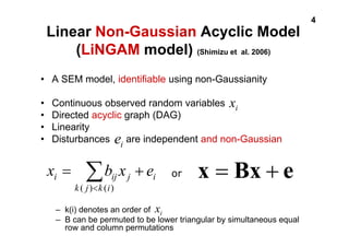
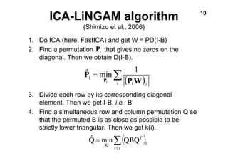
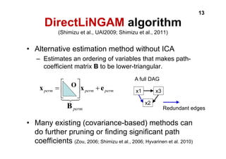
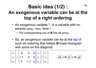
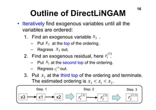
DirectLiNGAM is a new non-Gaussian estimation method for the LiNGAM model that directly estimates the variable ordering without using ICA. It iteratively identifies exogenous variables using independence tests between each variable and its residuals from regression on other variables. This allows it to estimate the ordering in a fixed number of steps, with no algorithmic parameters, convergence issues, or scale dependence like previous ICA-based methods. It was shown to estimate the correct causal ordering on a real-world socioeconomic dataset, matching domain knowledge better than alternative methods like ICA-LiNGAM, PC algorithm, and GES.

1. Updated at Jan 14 2011
DirectLiNGAM:
A direct estimation method for
LiNGAM
Shohei Shimizu, Takanori Inazumi, Yasuhiro Sogawa, Osaka Univ.
Aapo Hyvarinen, Univ. Helsinki
Yoshinobu Kawahara, Takashi Washio, Osaka Univ.
Patrik O. Hoyer, Univ. Helsinki
Kenneth Bollen, Univ. North Carolina

2. 2
Abstract
• Structural equation models (SEMs) are widely
used in many empirical sciences (Bollen, 1989)
• A non-Gaussian framework has been shown to
be useful for discovering SEMs (Shimizu, et al. 2006)
• Propose a new non-Gaussian estimation method
– No algorithmic parameters
– Guaranteed convergence in a fixed number of steps
if the data strictly follows the model

3. Background

4. 4
Linear Non-Gaussian Acyclic Model
(LiNGAM model) (Shimizu et al. 2006)
• A SEM model, identifiable using non-Gaussianity
• Continuous observed random variables
x
i • Directed acyclic graph (DAG)
• Linearity
• Disturbances are independent and non-Gaussian
x = Bx + e i
i e
i ij j e x b x + = Σ<
k j k i
( ) ( )
or
i x
– k(i) denotes an order of
– B can be permuted to be lower triangular by simultaneous equal
row and column permutations

5. 5
⎤
x
1
2
x
-1.3
Example
• A three-variable model
x =
e
1 1
x = 1.5
x +
e
2 1 2
x = − 1.3
x +
e
3 2 3
• Orders of variables:
⎡
⎤
⎡
x
1
2
0 0 0
1.5 0 0
x
–
– x2 can be influenced by x1, but never by x3
• External influences:
– x1 is equal to e1 and is exogenous
– e2 and e3 are errors
⎤
⎥ ⎥ ⎥
⎦
⎡
+
⎢ ⎢ ⎢
⎣
⎥ ⎥ ⎥
⎦
⎡
⎢ ⎢ ⎢
⎣
⎤
⎥ ⎥ ⎥
⎦
⎢ ⎢ ⎢
⎣
−
=
⎥ ⎥ ⎥
⎦
⎢ ⎢ ⎢
⎣
e
1
e
2
3
3
3
0 1.3 0
e
x
x
1442443
k(1) =1, k(2) = 2, k(3) = 3
x3
x1
x2
1.5
e1
e2 e3
B

6. 6
Our goal
• We know
– Data X is generated by
• We do NOT know
x = Bx + e
ij b
– Connection strengths:
– Orders: k(i)
– Disturbances:
• What we observe is data X only
• Goal
i e
– Estimate B and k using data X only!

7. Previous work

8. 8 Independent Component Analysis
(Comon 1994; Hyvarinen et al., 2001)
x = As
• A is an unknown square matrix
• are independent and non-Gaussian
i s
• Identifiable including the rotation (Comon, 1994)
• Many estimation methods
– e.g., FastICA (Hyvarinen,99), Amari (99) and Bach & Jordan (02)

9. 9 Key idea
i x
• Observed variables are linear combinations of
non-Gaussian independent disturbances
• ICA gives
x = Bx +
e
( )−1
x I B e
⇒ = −
Ae
=
-- ICA!
W= PDA−1 = PD(I −B)
– P: Permutation matrix, D: scaling matrix
i e
• Permutation indeterminacy in ICA can be solved
– Can be shown that the correct permutation is the only one which
has no zeros in the diagonal (Shimizu et al., UAI2005)

10. ICA-LiNGAM algorithm 10
(Shimizu et al., 2006)
1. Do ICA (here, FastICA) and get W = PD(I-B)
2. Find a permutation that gives no zeros on the
diagonal. Then we obtain D(I-B).
ˆ min 1
= Σ ( )
i ii PW
P
P
1
1
1
3. Divide each row by its corresponding diagonal
element. Then we get I-B, i.e., B
4. Find a simultaneous row and column permutation Q so
that the permuted B is as close as possible to be
strictly lower triangular. Then we get k(i).
( ) Σ≤
ˆ =
min
i j
ij
Q QBQT
Q
1 P

11. 11 Potential problems of
ICA-LiNGAM algorithm
1. ICA is an iterative search method
– May stuck in a local optimum if the initial
guess or step size is badly chosen
2. The permutation algorithms are not
scale-invariant
– May provide different variable orderings for
different scales of variables

12. A new method

13. 13
DirectLiNGAM algorithm
(Shimizu et al., UAI2009; Shimizu et al., 2011)
• Alternative estimation method without ICA
– Estimates an ordering of variables that makes path-coefficient
matrix B to be lower-triangular.
perm perm perm e x x + ⎥⎦ ⎤
⎡
=
123
⎢⎣
O
perm B
A full DAG
x1 x3
x2
Redundant edges
• Many existing (covariance-based) methods can
do further pruning or finding significant path
coefficients (Zou, 2006; Shimizu et al., 2006; Hyvarinen et al. 2010)

14. Basic idea (1/2) : 14
An exogenous variable can be at the
top of a right ordering
• An exogenous variable is a variable with no
parents (Bollen, 1989), here .
– The corresponding row of B has all zeros.
• So, an exogenous variable can be at the top of
such an ordering that makes B lower-triangular
with zeros on the diagonal.
⎤
⎥ ⎥ ⎥
⎦
⎡
+
⎢ ⎢ ⎢
⎣
⎤
⎥ ⎥ ⎥
⎦
⎡
⎢ ⎢ ⎢
⎣
⎤
⎥ ⎥ ⎥
⎦
⎡
⎢ ⎢ ⎢
0 0 0
1.5 0 ⎣
−
=
⎤
⎥ ⎥ ⎥
⎦
⎡
⎢ ⎢ ⎢
⎣
e
3
e
1
2
x
3
x
1
2
x
3
x
1
2
0 1.3 0
e
x
x
0
0
0
0
0 0
x3 x1 x2
j x
3 x

15. Basic idea (2/2): 15
3 x
Regress exogenous out
r(3) (i =1,2) i
• Compute the residuals regressing the other
variables on exogenous :
3 x (i =1,2) x i
( ) (3)
3
1 r and r
– The residuals form a LiNGAM model.
– The ordering of the residuals is equivalent to that of
corresponding original variables.
⎤
⎥ ⎥ ⎥
⎦
⎡
+
⎢ ⎢ ⎢
⎣
⎤
⎥ ⎥ ⎥
⎦
⎡
⎢ ⎢ ⎢
⎣
⎤
⎥ ⎥ ⎥
⎦
2
e
3
e
1
e
2
x
3
x
1
2
0 0
x
0
0
0
0
1 r 1 x
x ⎡
0
⎢ ⎢ ⎢
1.5 0 ⎣
0
0 −
1.3 =
⎤
⎥ ⎥ ⎥
⎦
⎡
⎢ ⎢ ⎢
⎣
3
x
1
2
x
⎡
+ ⎥⎦
⎡
r 0 0
⎤
⎡
−
⎤
⎡
(3)
1
(3)
1
r
• Exogenous ( 3 ) implies ` can be at the second top’.
⎤
⎥⎦
⎢⎣
⎤
⎢⎣
⎥⎦
⎢⎣
= ⎥⎦
⎢⎣
e
1
2
(3)
2
(3)
2
1.3 e
r
r
(3)
2 (3) r
1 x3 x1 x2 r
0

16. 16
Outline of DirectLiNGAM
• Iteratively find exogenous variables until all the
variables are ordered:
1. Find an exogenous variable .
– Put at the top of the ordering.
– Regress out.
2. Find an exogenous residual, here .
– Put at the second top of the ordering.
– Regress out.
3. Put at the third top of the ordering and terminate.
The estimated ordering is
3 x
(3)
1 r
3 x
1 x3 x1 x2 r (3,1)
2 r
(3)
2 (3) r
3 x
1 x
(3)
1 r
2 x
. 3 1 2 x < x < x
Step. 1 Step. 2 Step. 3

17. 17
Identification of an exogenous
variable (two variable cases)
i) is exogenous. ii) is NOT exogenous.
( )
1 e
x b x b
=
1 = 12 2 + 12 ≠
0
x e
x b var
x
12 2
var( )
x x
( ) 1 1 x = e 1 x
Regressing on ,
r x x x
cov( , )
2 1
var( )
= −
b x x
1 12 cov( 2 , 1
)
var( )
1
2
1
1
1
2
(1)
2
2 1
x
x
x
x
−
⎭ ⎬ ⎫
⎩ ⎨ ⎧
= −
x e
=
x b x e b
1 1
= + ≠
( 0) 2 21 1 2 21
x x
Regressing on ,
r x x x
cov( , )
= −
x b x
= −
2 21 1
2
1
2 1
1
2
(1)
2
2 1
var( )
e
x
x
=
( )
2 2
1 e
and (1) are NOT independent.
1 2 and (1) are independent. x r
1 2 x r

18. Need to use Darmois-Skitovitch’ 18
theorem (Darmois, 1953; Skitovitch, 1953)
( )
1
x b x e b
=
1 = 12 2 + ⋅ 1 12 ≠
0
x e
x x
1
2
2
x x
Regressing on ,
r x x x
cov( , )
2 1
var( )
= −
b x x
1 12 cov( 2 , 1
)
1
1
1
2
(1)
2
1 2
var
var( )
var( )
e
x
x
x
x
−
⎭ ⎬ ⎫
⎩ ⎨ ⎧
= −
( )
2 2
Darmois-Skitovitch’ theorem:
Define two variables and as
ii) 1 is NOT exogenous. x
and (1) are NOT independent.
1 2 x r
Σ Σ
= =
x 1 = a 1 j e j ,
x =
a e
p
2 2
j
j j
p
j
1
1
1 x
j e
where are independent
random variables.
If there exists a non-Gaussian
for which ,
and are dependent.
i e
0 1 2 ≠ i i a a
1 x 2 x
1
12 b
2 x

19. 19
Identification of an exogenous
variable (p variable cases)
( )
cov( ) x
j = − , x x
i j
j
i x
r x
• Lemma 1: and its residual
are independent for all is exogenous
j
var( )
j
i
x
i ≠ j j ⇔ x
• In practice, we can identify an exogenous variable
by finding a variable that is most independent of
its residuals

20. 20 Independence measures
• Evaluate independence between a variable and a
residual by a nonlinear correlation:
corr{x , g(r( j) )} (g = tanh)
j i
• Taking the sum over all the residuals, we get:
{ ( j
Σ≠
) } { ( ) } T = corr x ) )
j , g i r( +
corr g x , r( i j
j
j i
• Can use more sophisticated measures as well
(Bach & Jordan, 2002; Gretton et al., 2005; Kraskov et al., 2004).
– Kernel-based independence measure (Bach & Jordan, 2002)
often gives more accurate estimates (Sogawa et al., IJCNN10)

21. Real-world data example (1/2) 21
• Status attainment model
– General Social Survey (U.S.A.)
– Sample size = 1380
• Non-farm, ages 35-45, white, male, in the labor force, years 1972-2006
Domain knowledge
(Duncan et al. 1972)
DirectLiNGAM

22. Real-world data example (2/2)
ICA-LiNGAM
PC algorithm GES
22

23. 23
Summary
• DirectLiNGAM repeats:
– Least squares simple linear regression
– Evaluation of pairwise independence between each
variable and its residuals
• No algorithmic parameters like stepsize, initial
guesses, convergence criteria
• Guaranteed convergence to the right solution in
a fixed number of steps (the number of
variables) if the data strictly follows the model