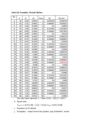
Download to read offline
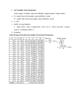
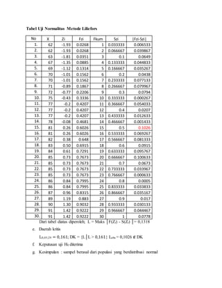

Dokumen ini menjelaskan uji normalitas pada kelas eksperimen dan kelas kontrol dengan menggunakan metode Liliefors. Hasil analisis menunjukkan bahwa pada kedua kelas, nol hipotesis (H0) diterima, yang berarti sampel berasal dari populasi yang berdistribusi normal. Rata-rata dan standar deviasi masing-masing kelas juga dihitung dan diperbandingkan.


![StatPen_kel_3_revisi[2].pptx selamat mencoba](https://cdn.slidesharecdn.com/ss_thumbnails/statpenkel3revisi2-250513155131-78ec9c78-thumbnail.jpg?width=640&height=640&fit=bounds)