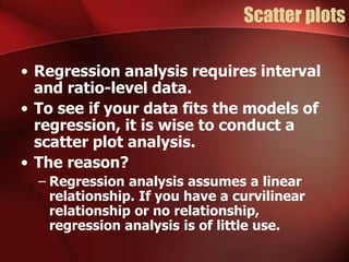
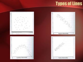
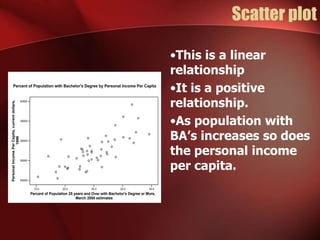
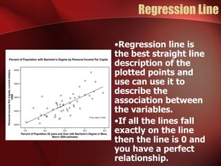
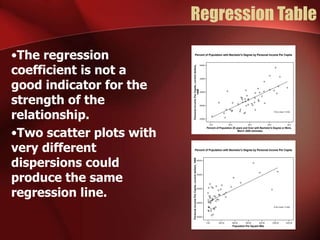
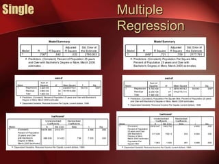
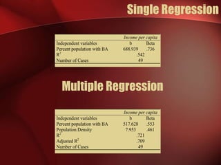
Regression analysis can be used to analyze the relationship between variables. A scatter plot should first be created to determine if the variables have a linear relationship required for regression analysis. A regression line is fitted to best describe the linear relationship between the variables, with an R-squared value indicating how well it fits the data. Multiple regression allows for analysis of the relationship between a dependent variable and multiple independent variables and their individual contributions to explaining the variance in the dependent variable.

1. Regression Analysis

2. Scatter plots
• Regression analysis requires interval
and ratio-level data.
• To see if your data fits the models of
regression, it is wise to conduct a
scatter plot analysis.
• The reason?
– Regression analysis assumes a linear
relationship. If you have a curvilinear
relationship or no relationship,
regression analysis is of little use.

3. Types of Lines

4. Scatter plot
15.0 20.0 25.0 30.0 35.0
Percent of Population 25 years and Over with Bachelor's Degree or More,
March 2000 estimates
20000
25000
30000
35000
40000
Personal
Income
Per
Capita,
current
dollars,
1999
Percent of Population with Bachelor's Degree by Personal Income Per Capita
•This is a linear
relationship
•It is a positive
relationship.
•As population with
BA’s increases so does
the personal income
per capita.

5. Regression Line
15.0 20.0 25.0 30.0 35.0
Percent of Population 25 years and Over with Bachelor's Degree or More,
March 2000 estimates
20000
25000
30000
35000
40000
Personal
Income
Per
Capita,
current
dollars,
1999
Percent of Population with Bachelor's Degree by Personal Income Per Capita
R Sq Linear = 0.542
•Regression line is
the best straight line
description of the
plotted points and
use can use it to
describe the
association between
the variables.
•If all the lines fall
exactly on the line
then the line is 0 and
you have a perfect
relationship.

6. Things to remember
• Regressions are still focuses on
association, not causation.
• Association is a necessary
prerequisite for inferring causation,
but also:
1. The independent variable must preceded
the dependent variable in time.
2. The two variables must be plausibly lined
by a theory,
3. Competing independent variables must
be eliminated.

7. Regression Table
•The regression
coefficient is not a
good indicator for the
strength of the
relationship.
•Two scatter plots with
very different
dispersions could
produce the same
regression line.
15.0 20.0 25.0 30.0 35.0
Percent of Population 25 years and Over with Bachelor's Degree or More,
March 2000 estimates
20000
25000
30000
35000
40000
Personal
Income
Per
Capita,
current
dollars,
1999
Percent of Population with Bachelor's Degree by Personal Income Per Capita
R Sq Linear = 0.542
0.00 200.00 400.00 600.00 800.00 1000.00 1200.00
Population Per Square Mile
20000
25000
30000
35000
40000
Personal
Income
Per
Capita,
current
dollars,
1999
Percent of Population with Bachelor's Degree by Personal Income Per Capita
R Sq Linear = 0.463

8. Regression coefficient
• The regression coefficient is the slope of
the regression line and tells you what
the nature of the relationship between
the variables is.
• How much change in the independent
variables is associated with how much
change in the dependent variable.
• The larger the regression coefficient the
more change.

9. Pearson’s r
• To determine strength you look at how
closely the dots are clustered around the
line. The more tightly the cases are
clustered, the stronger the relationship,
while the more distant, the weaker.
• Pearson’s r is given a range of -1 to + 1
with 0 being no linear relationship at all.

10. Reading the tables
•When you run regression analysis on SPSS you get a
3 tables. Each tells you something about the
relationship.
•The first is the model summary.
•The R is the Pearson Product Moment Correlation
Coefficient.
•In this case R is .736
•R is the square root of R-Squared and is the
correlation between the observed and predicted
values of dependent variable.
Model Summary
.736a
.542 .532 2760.003
Model
1
R R Square
Adjusted
R Square
Std. Error of
the Estimate
Predictors: (Constant), Percent of Population 25 years
and Over with Bachelor's Degree or More, March 2000
estimates
a.

11. R-Square
•R-Square is the proportion of variance in the
dependent variable (income per capita) which can be
predicted from the independent variable (level of
education).
•This value indicates that 54.2% of the variance in
income can be predicted from the variable
education. Note that this is an overall measure of the
strength of association, and does not reflect the
extent to which any particular independent variable
is associated with the dependent variable.
•R-Square is also called the coefficient of
Model Summary
.736a
.542 .532 2760.003
Model
1
R R Square
Adjusted
R Square
Std. Error of
the Estimate
Predictors: (Constant), Percent of Population 25 years
and Over with Bachelor's Degree or More, March 2000
estimates
a.

12. Adjusted R-square
•As predictors are added to the model, each predictor will explain
some of the variance in the dependent variable simply due to
chance.
•One could continue to add predictors to the model which would
continue to improve the ability of the predictors to explain the
dependent variable, although some of this increase in R-square
would be simply due to chance variation in that particular sample.
•The adjusted R-square attempts to yield a more honest value to
estimate the R-squared for the population. The value of R-square
was .542, while the value of Adjusted R-square was .532. There
isn’t much difference because we are dealing with only one
variable.
•When the number of observations is small and the number of
predictors is large, there will be a much greater difference between
R-square and adjusted R-square.
•By contrast, when the number of observations is very large
compared to the number of predictors, the value of R-square and
Model Summary
.736a
.542 .532 2760.003
Model
1
R R Square
Adjusted
R Square
Std. Error of
the Estimate
Predictors: (Constant), Percent of Population 25 years
and Over with Bachelor's Degree or More, March 2000
estimates
a.

13. ANOVA
•The p-value associated with this F value is very small
(0.0000).
•These values are used to answer the question "Do the
independent variables reliably predict the dependent
variable?".
•The p-value is compared to your alpha level (typically 0.05)
and, if smaller, you can conclude "Yes, the independent
variables reliably predict the dependent variable".
•If the p-value were greater than 0.05, you would say that the
group of independent variables does not show a statistically
significant relationship with the dependent variable, or that
the group of independent variables does not reliably predict
the dependent variable.
ANOVAb
4.32E+08 1 432493775.8 56.775 .000a
3.66E+08 48 7617618.586
7.98E+08 49
Regression
Residual
Total
Model
1
Sum of
Squares df Mean Square F Sig.
Predictors: (Constant), Percent of Population 25 years and Over with Bachelor's
Degree or More, March 2000 estimates
a.
Dependent Variable: Personal Income Per Capita, current dollars, 1999
b.

14. Coefficients
•B - These are the values for the regression equation
for predicting the dependent variable from the
independent variable.
•These are called unstandardized coefficients
because they are measured in their natural
units. As such, the coefficients cannot be compared
with one another to determine which one is more
influential in the model, because they can be
measured on different scales.
Coefficientsa
10078.565 2312.771 4.358 .000
688.939 91.433 .736 7.535 .000
(Constant)
Percent of Population
25 years and Over
with Bachelor's
Degree or More,
March 2000 estimates
Model
1
B Std. Error
Unstandardized
Coefficients
Beta
Standardized
Coefficients
t Sig.
Dependent Variable: Personal Income Per Capita, current dollars, 1999
a.

15. Coefficients
•This chart looks at two variables and shows how
the different bases affect the B value. That is why
you need to look at the standardized Beta to see
the differences.
Coefficientsa
13032.847 1902.700 6.850 .000
517.628 78.613 .553 6.584 .000
7.953 1.450 .461 5.486 .000
(Constant)
Percent of Population
25 years and Over
with Bachelor's
Degree or More,
March 2000 estimates
Population Per
Square Mile
Model
1
B Std. Error
Unstandardized
Coefficients
Beta
Standardized
Coefficients
t Sig.
Dependent Variable: Personal Income Per Capita, current dollars, 1999
a.

16. Coefficients
•Beta - The are the standardized coefficients.
•These are the coefficients that you would obtain if you
standardized all of the variables in the regression, including
the dependent and all of the independent variables, and ran
the regression.
•By standardizing the variables before running the regression,
you have put all of the variables on the same scale, and you
can compare the magnitude of the coefficients to see which
one has more of an effect.
•You will also notice that the larger betas are associated with
Coefficientsa
10078.565 2312.771 4.358 .000
688.939 91.433 .736 7.535 .000
(Constant)
Percent of Population
25 years and Over
with Bachelor's
Degree or More,
March 2000 estimates
Model
1
B Std. Error
Unstandardized
Coefficients
Beta
Standardized
Coefficients
t Sig.
Dependent Variable: Personal Income Per Capita, current dollars, 1999
a.

17. How to translate a typical table
Regression Analysis Level of Education by Income per capita
Income per capita
Independent variables b Beta
Percent population with BA 688.939 .736
R2
.542
Number of Cases 49

18. Part of the Regression Equation
• b represents the slope of the line
– It is calculated by dividing the change in
the dependent variable by the change in
the independent variable.
– The difference between the actual value
of Y and the calculated amount is called
the residual.
– The represents how much error there is
in the prediction of the regression
equation for the y value of any
individual case as a function of X.

19. Comparing two variables
• Regression analysis is useful for
comparing two variables to see whether
controlling for other independent variable
affects your model.
• For the first independent variable,
education, the argument is that a more
educated populace will have higher-paying
jobs, producing a higher level of per capita
income in the state.
• The second independent variable is
included because we expect to find better-
paying jobs, and therefore more
opportunity for state residents to obtain
them, in urban rather than rural areas.

20. Single
Model Summary
.849a
.721 .709 2177.791
Model
1
R R Square
Adjusted
R Square
Std. Error of
the Estimate
Predictors: (Constant), Population Per Square Mile,
Percent of Population 25 years and Over with
Bachelor's Degree or More, March 2000 estimates
a.
ANOVAb
5.75E+08 2 287614518.2 60.643 .000a
2.23E+08 47 4742775.141
7.98E+08 49
Regression
Residual
Total
Model
1
Sum of
Squares df Mean Square F Sig.
Predictors: (Constant), Population Per Square Mile, Percent of Population 25 years
and Over with Bachelor's Degree or More, March 2000 estimates
a.
Dependent Variable: Personal Income Per Capita, current dollars, 1999
b.
Coefficientsa
13032.847 1902.700 6.850 .000
517.628 78.613 .553 6.584 .000
7.953 1.450 .461 5.486 .000
(Constant)
Percent of Population
25 years and Over
with Bachelor's
Degree or More,
March 2000 estimates
Population Per
Square Mile
Model
1
B Std. Error
Unstandardized
Coefficients
Beta
Standardized
Coefficients
t Sig.
Dependent Variable: Personal Income Per Capita, current dollars, 1999
a.
Model Summary
.736a
.542 .532 2760.003
Model
1
R R Square
Adjusted
R Square
Std. Error of
the Estimate
Predictors: (Constant), Percent of Population 25 years
and Over with Bachelor's Degree or More, March 2000
estimates
a.
ANOVAb
4.32E+08 1 432493775.8 56.775 .000a
3.66E+08 48 7617618.586
7.98E+08 49
Regression
Residual
Total
Model
1
Sum of
Squares df Mean Square F Sig.
Predictors: (Constant), Percent of Population 25 years and Over with Bachelor's
Degree or More, March 2000 estimates
a.
Dependent Variable: Personal Income Per Capita, current dollars, 1999
b.
Coefficientsa
10078.565 2312.771 4.358 .000
688.939 91.433 .736 7.535 .000
(Constant)
Percent of Population
25 years and Over
with Bachelor's
Degree or More,
March 2000 estimates
Model
1
B Std. Error
Unstandardized
Coefficients
Beta
Standardized
Coefficients
t Sig.
Dependent Variable: Personal Income Per Capita, current dollars, 1999
a.
Multiple
Regression

21. Single Regression
Income per capita
Independent variables b Beta
Percent population with BA 688.939 .736
R2
.542
Number of Cases 49
Multiple Regression
Income per capita
Independent variables b Beta
Percent population with BA 517.628 .553
Population Density 7.953 .461
R2
.721
Adjusted R2
.709
Number of Cases 49

22. Perceptions of victory

23. Regression