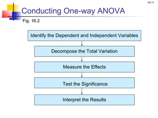
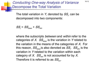
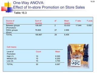
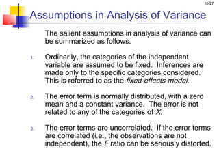
This chapter outline describes one-way analysis of variance (ANOVA). It introduces key concepts like decomposing total variation into between- and within-group components to test if group means are equal. The chapter will cover conducting a one-way ANOVA, including identifying variables, decomposing variation, measuring effects with statistics like η2, testing significance with the F-ratio, and interpreting results. Examples and assumptions of one-way ANOVA will also be discussed.

1. Chapter Sixteen
Analysis of Variance and
Covariance

2. 16-2
Chapter Outline
1) Overview
2) Relationship Among Techniques
2) One-Way Analysis of Variance
3) Statistics Associated with One-Way Analysis of Variance
4) Conducting One-Way Analysis of Variance
i. Identification of Dependent & Independent
Variables
ii. Decomposition of the Total Variation
iii. Measurement of Effects
iv. Significance Testing
v. Interpretation of Results

3. 16-3
Chapter Outline
5) Illustrative Data
6) Illustrative Applications of One-Way Analysis of
Variance
7) Assumptions in Analysis of Variance
8) N-Way Analysis of Variance
9) Analysis of Covariance
10) Issues in Interpretation
i. Interactions
ii. Relative Importance of Factors
iii. Multiple Comparisons
6) Repeated Measures ANOVA

4. 16-4
Chapter Outline
12) Nonmetric Analysis of Variance
13) Multivariate Analysis of Variance
14) Internet and Computer Applications
15) Focus on Burke
16) Summary
17) Key Terms and Concepts

5. 16-5
Relationship Among Techniques
 Analysis of variance (ANOVA) is used as a test
of means for two or more populations. The null
hypothesis, typically, is that all means are equal.
 Analysis of variance must have a dependent variable
that is metric (measured using an interval or ratio
scale).
 There must also be one or more independent
variables that are all categorical (nonmetric).
Categorical independent variables are also called
factors.

6. 16-6
Relationship Among Techniques
 A particular combination of factor levels, or
categories, is called a treatment.
 One-way analysis of variance involves only one
categorical variable, or a single factor. In one-way
analysis of variance, a treatment is the same as a
factor level.
 If two or more factors are involved, the analysis is
termed n -way analysis of variance .
 If the set of independent variables consists of both
categorical and metric variables, the technique is
called analysis of covariance (ANCOVA) . In
this case, the categorical independent variables are
still referred to as factors, whereas the metric-
independent variables are referred to as covariates.

7. Relationship Amongst Test, Analysis of
16-7
Variance, Analysis of Covariance, & Regression
Fig. 16.1
Metric Dependent Variable
One Variable
Independent Independent More
One or Variables
Categorical: Categorical
Binary Interval
Factorial and Interval
Analysis of Analysis of
t Test Variance Covariance Regression
More than
One Factor One Factor
One-Way Analysis N-Way Analysis
of Variance of Variance

8. 16-8
One-way Analysis of Variance
Marketing researchers are often interested in
examining the differences in the mean values of the
dependent variable for several categories of a single
independent variable or factor. For example:
 Do the various segments differ in terms of their
volume of product consumption?
 Do the brand evaluations of groups exposed to
different commercials vary?
 What is the effect of consumers' familiarity with the
store (measured as high, medium, and low) on
preference for the store?

9. Statistics Associated with One-way
16-9
Analysis of Variance
 eta 2 ( η). The strength of the effects of X
2
(independent variable or factor) on Y (dependent
variable) is measured by eta 2 ( η). The value of η
2 2
varies between 0 and 1.
 F statistic. The null hypothesis that the category
means are equal in the population is tested by an F
statistic based on the ratio of mean square related
to X and mean square related to error.
 Mean square. This is the sum of squares divided
by the appropriate degrees of freedom.

10. Statistics Associated with One-way
16-10
Analysis of Variance
 SS between . Also denoted as SS x , this is the variation in
Y related to the variation in the means of the
categories of X. This represents variation between
the categories of X, or the portion of the sum of
squares in Y related to X.
 SS within . Also referred to as SS error , this is the variation
in Y due to the variation within each of the categories
of X. This variation is not accounted for by X.
 SS y . This is the total variation in Y.

11. 16-11
Conducting One-way ANOVA
Fig. 16.2
Identify the Dependent and Independent Variables
Decompose the Total Variation
Measure the Effects
Test the Significance
Interpret the Results

12. Conducting One-way Analysis of Variance 16-12
Decompose the Total Variation
The total variation in Y, denoted by SSy, can be
decomposed into two components:
SSy = SSbetween + SSwithin
where the subscripts between and within refer to the
categories of X. SSbetween is the variation in Y related to
the variation in the means of the categories of X. For
this reason, SSbetween is also denoted as SSx. SSwithin is the
variation in Y related to the variation within each
category of X. SSwithin is not accounted for by X.
Therefore it is referred to as SSerror.

13. Conducting One-way Analysis of Variance 16-13
Decompose the Total Variation
The total variation in Y may be decomposed as:
SSy = SSx + SSerror
where
N
SSy = Σ (Y i - 2)
Y
i =1
c
S Sx = Σ n ( j - )2
Y Y
j =1
c n
SS error= Σ Σ (Y ij -Y j )2
j i
Yi = individual observation
Y
j = mean for category j
Y = mean over the whole sample, or grand mean
Yij = i th observation in the j th category

14. Decomposition of the Total Variation:
16-14
One-way ANOVA
Table 16.1
Independent Variable X
Total
Categories Sample
Within X1 X2 X3 … Xc
Category Y1 Y1 Y1 Y1 Y1 Total
Variation Variation
=SSwithin Y2 Y2 Y2 Y2 Y2 =SSy
: :
: :
Yn Yn Yn Yn YN
Category
Mean Y1 Y2 Y3 Yc Y
Between Category Variation = SSbetween

15. 16-15
Conducting One-way Analysis of Variance
In analysis of variance, we estimate two measures of
variation: within groups (SSwithin) and between groups
(SSbetween). Thus, by comparing the Y variance
estimates based on between-group and within-group
variation, we can test the null hypothesis.
Measure the Effects
The strength of the effects of X on Y are measured
as follows:
η = SS /SS = (SS - SS )/SS
2
x y y error y
η
The value of 2 varies between 0 and 1.

16. Conducting One-way Analysis of Variance 16-16
Test Significance
In one-way analysis of variance, the interest lies in testing the null
hypothesis that the category means are equal in the population.
H0: µ1 = µ2 = µ3 = ........... = µc
Under the null hypothesis, SSx and SSerror come from the same source of
variation. In other words, the estimate of the population variance of Y,
2 = SSx/(c - 1)
S y
= Mean square due to X
= MSx
or
2
= SSerror/(N - c)
S y
= Mean square due to error
= MSerror

17. Conducting One-way Analysis of Variance 16-17
Test Significance
The null hypothesis may be tested by the F statistic
based on the ratio between these two estimates:
SS x /(c - 1) MS x
F= =
SS error/(N - c) MS error
This statistic follows the F distribution, with (c - 1) and
(N - c) degrees of freedom (df).

18. Conducting One-way Analysis of Variance 16-18
Interpret the Results
 If the null hypothesis of equal category means is not
rejected, then the independent variable does not
have a significant effect on the dependent variable.
 On the other hand, if the null hypothesis is rejected,
then the effect of the independent variable is
significant.
 A comparison of the category mean values will
indicate the nature of the effect of the independent
variable.

19. Illustrative Applications of One-way
16-19
Analysis of Variance
We illustrate the concepts discussed in this chapter
using the data presented in Table 16.2.
The department store is attempting to determine the
effect of in-store promotion (X) on sales (Y). For the
purpose of illustrating hand calculations, the data of
Table 16.2 are transformed in Table 16.3 to show the
store sales (Yij) for each level of promotion.
The null hypothesis is that the category means are
equal:
H0: µ1 = µ2 = µ3.

20. Effect of Promotion and Clientele on 16-20
Sales
Table 16.2
Store Num ber Coupon Level In-Store Prom otion Sales Clientel Rating
1 1.00 1.00 10.00 9.00
2 1.00 1.00 9.00 10.00
3 1.00 1.00 10.00 8.00
4 1.00 1.00 8.00 4.00
5 1.00 1.00 9.00 6.00
6 1.00 2.00 8.00 8.00
7 1.00 2.00 8.00 4.00
8 1.00 2.00 7.00 10.00
9 1.00 2.00 9.00 6.00
10 1.00 2.00 6.00 9.00
11 1.00 3.00 5.00 8.00
12 1.00 3.00 7.00 9.00
13 1.00 3.00 6.00 6.00
14 1.00 3.00 4.00 10.00
15 1.00 3.00 5.00 4.00
16 2.00 1.00 8.00 10.00
17 2.00 1.00 9.00 6.00
18 2.00 1.00 7.00 8.00
19 2.00 1.00 7.00 4.00
20 2.00 1.00 6.00 9.00
21 2.00 2.00 4.00 6.00
22 2.00 2.00 5.00 8.00
23 2.00 2.00 5.00 10.00
24 2.00 2.00 6.00 4.00
25 2.00 2.00 4.00 9.00
26 2.00 3.00 2.00 4.00
27 2.00 3.00 3.00 6.00
28 2.00 3.00 2.00 10.00
29 2.00 3.00 1.00 9.00
30 2.00 3.00 2.00 8.00

21. Illustrative Applications of One-way
16-21
Analysis of Variance
TABLE 16.3
EFFECT OF IN-STORE PROMOTION ON SALES
Store Level of In-store Promotion
No. High Medium Low
Normalized Sales
_________________
1 10 8 5
2 9 8 7
3 10 7 6
4 8 9 4
5 9 6 5
6 8 4 2
7 9 5 3
8 7 5 2
9 7 6 1
10 6 4 2
_____________________________________________________
Column Totals Y 83 62 37
Category means: j 83/10 62/10 37/10
Y = 8.3 = 6.2 = 3.7

22. Illustrative Applications of One-way
16-22
Analysis of Variance
To test the null hypothesis, the various sums of squares are computed as follows:
SSy = (10-6.067)2 + (9-6.067)2 + (10-6.067)2 + (8-6.067)2 + (9-6.067)2
+ (8-6.067)2 + (9-6.067)2 + (7-6.067)2 + (7-6.067)2 + (6-6.067)2
+ (8-6.067)2 + (8-6.067)2 + (7-6.067)2 + (9-6.067)2 + (6-6.067)2
(4-6.067)2 + (5-6.067)2 + (5-6.067)2 + (6-6.067)2 + (4-6.067)2
+ (5-6.067)2 + (7-6.067)2 + (6-6.067)2 + (4-6.067)2 + (5-6.067)2
+ (2-6.067)2 + (3-6.067)2 + (2-6.067)2 + (1-6.067)2 + (2-6.067)2
=(3.933)2 + (2.933)2 + (3.933)2 + (1.933)2 + (2.933)2
+ (1.933)2 + (2.933)2 + (0.933)2 + (0.933)2 + (-0.067)2
+ (1.933)2 + (1.933)2 + (0.933)2 + (2.933)2 + (-0.067)2
(-2.067)2 + (-1.067)2 + (-1.067)2 + (-0.067)2 + (-2.067)2
+ (-1.067)2 + (0.9333)2 + (-0.067)2 + (-2.067)2 + (-1.067)2
+ (-4.067)2 + (-3.067)2 + (-4.067)2 + (-5.067)2 + (-4.067)2
= 185.867

23. Illustrative Applications of One-way
16-23
Analysis of Variance (cont.)
SSx = 10(8.3-6.067)2 + 10(6.2-6.067)2 + 10(3.7-6.067)2
= 10(2.233)2 + 10(0.133)2 + 10(-2.367)2
= 106.067
SSerror = (10-8.3)2 + (9-8.3)2 + (10-8.3)2 + (8-8.3)2 + (9-8.3)2
+ (8-8.3)2 + (9-8.3)2 + (7-8.3)2 + (7-8.3)2 + (6-8.3)2
+ (8-6.2)2 + (8-6.2)2 + (7-6.2)2 + (9-6.2)2 + (6-6.2)2
+ (4-6.2)2 + (5-6.2)2 + (5-6.2)2 + (6-6.2)2 + (4-6.2)2
+ (5-3.7)2 + (7-3.7)2 + (6-3.7)2 + (4-3.7)2 + (5-3.7)2
+ (2-3.7)2 + (3-3.7)2 + (2-3.7)2 + (1-3.7)2 + (2-3.7)2
= (1.7)2 + (0.7)2 + (1.7)2 + (-0.3)2 + (0.7)2
+ (-0.3)2 + (0.7)2 + (-1.3)2 + (-1.3)2 + (-2.3)2
+ (1.8)2 + (1.8)2 + (0.8)2 + (2.8)2 + (-0.2)2
+ (-2.2)2 + (-1.2)2 + (-1.2)2 + (-0.2)2 + (-2.2)2
+ (1.3)2 + (3.3)2 + (2.3)2 + (0.3)2 + (1.3)2
+ (-1.7)2 + (-0.7)2 + (-1.7)2 + (-2.7)2 + (-1.7)2
= 79.80

24. Illustrative Applications of One-way
16-24
Analysis of Variance
It can be verified that
SSy = SSx + SSerror
as follows:
185.867 = 106.067 +79.80
The strength of the effects of X on Y are measured as follows:
η2 = SSx/SSy
= 106.067/185.867
= 0.571
In other words, 57.1% of the variation in sales (Y) is accounted
for by in-store promotion (X), indicating a modest effect. The
null hypothesis may now be tested.
F = SS error/(N - c) = MS error
SS x /(c - 1) MS X
106.067/(3-1)
F=
79.800/(30-3)
= 17.944

25. Illustrative Applications of One-way
16-25
Analysis of Variance
 From Table 5 in the Statistical Appendix we see that
for 2 and 27 degrees of freedom, the critical value of
F is 3.35 for α = 0.05 Because the calculated value
.
of F is greater than the critical value, we reject the
null hypothesis.
 We now illustrate the analysis of variance procedure
using a computer program. The results of conducting
the same analysis by computer are presented in
Table 16.4.

26. One-Way ANOVA:
16-26
Effect of In-store Promotion on Store Sales
Table 16.3
Source of Sum of df Mean F ratio F prob.
Variation squares square
Between groups 106.067 2 53.033 17.944 0.000
(Promotion)
Within groups 79.800 27 2.956
(Error)
TOTAL 185.867 29 6.409
Cell means
Level of Count Mean
Promotion
High (1) 10 8.300
Medium (2) 10 6.200
Low (3) 10 3.700
TOTAL 30 6.067

27. 16-27
Assumptions in Analysis of Variance
The salient assumptions in analysis of variance can
be summarized as follows.
1. Ordinarily, the categories of the independent
variable are assumed to be fixed. Inferences are
made only to the specific categories considered.
This is referred to as the fixed-effects model.
2. The error term is normally distributed, with a zero
mean and a constant variance. The error is not
related to any of the categories of X.
3. The error terms are uncorrelated. If the error terms
are correlated (i.e., the observations are not
independent), the F ratio can be seriously distorted.

28. 16-28
N-way Analysis of Variance
In marketing research, one is often concerned with the
effect of more than one factor simultaneously. For
example:
 How do advertising levels (high, medium, and low) interact
with price levels (high, medium, and low) to influence a
brand's sale?
 Do educational levels (less than high school, high school
graduate, some college, and college graduate) and age
(less than 35, 35-55, more than 55) affect consumption of
a brand?
 What is the effect of consumers' familiarity with a
department store (high, medium, and low) and store
image (positive, neutral, and negative) on preference for
the store?

29. 16-29
N-way Analysis of Variance
Consider the simple case of two factors X1 and X2 having categories c1
and c2. The total variation in this case is partitioned as follows:
SStotal = SS due to X1 + SS due to X2 + SS due to interaction of X1 and X2
+ SSwithin
or
SS y = SS x 1 + SS x 2 + SS x 1x 2 + SS error
The strength of the joint effect of two factors, called the overall effect, or
multiple
η measured as follows:
2
, is
multiple
η (SS x 1 + SS x 2 + SS x 1x 2)/ SS y
2
=

30. 16-30
N-way Analysis of Variance
The significance of the overall effect may be tested by an F test,
as follows
(SS x 1 + SS x 2 + SS x 1x 2)/dfn
F=
SS error/dfd
SS x 1,x 2,x 1x 2/ dfn
=
SS error/dfd
MS x 1,x 2,x 1x 2
=
MS error
where
dfn = degrees of freedom for the numerator
= (c1 - 1) + (c2 - 1) + (c1 - 1) (c2 - 1)
= c1c2 - 1
dfd = degrees of freedom for the denominator
= N - c1c2
MS = mean square

31. 16-31
N-way Analysis of Variance
If the overall effect is significant, the next step is to examine the
significance of the interaction effect. Under the null
hypothesis of no interaction, the appropriate F test is:
SS x 1x 2/dfn
F=
SS error/dfd
MS x 1x 2
=
MS error
where
dfn = (c1 - 1) (c2 - 1)
dfd = N - c1c2

32. 16-32
N-way Analysis of Variance
The significance of the main effect of each factor may
be tested as follows for X1:
SS x 1/dfn
F=
SS error/dfd
MS x 1
=
MS error
where
dfn = c1 - 1
dfd = N - c1c2

33. 16-33
Two-way Analysis of Variance
Table 16.4
Source of Sum of Mean Sig. of
Variation squares df square F F ω2
Main Effects
Promotion 106.067 2 53.033 54.862 0.000 0.557
Coupon 53.333 1 53.333 55.172 0.000 0.280
Combined 159.400 3 53.133 54.966 0.000
Two-way 3.267 2 1.633 1.690 0.226
interaction
Model 162.667 5 32.533 33.655 0.000
Residual (error) 23.200 24 0.967
TOTAL 185.867 29 6.409

34. 16-34
Two-way Analysis of Variance
Table 16.4 cont.
Cell Means
Promotion Coupon Count Mean
High Yes 5 9.200
High No 5 7.400
Medium Yes 5 7.600
Medium No 5 4.800
Low Yes 5 5.400
Low No 5 2.000
TOTAL 30
Factor Level
Means
Promotion Coupon Count Mean
High 10 8.300
Medium 10 6.200
Low 10 3.700
Yes 15 7.400
No 15 4.733
Grand Mean 30 6.067

35. 16-35
Analysis of Covariance
When examining the differences in the mean values of the
dependent variable related to the effect of the controlled
independent variables, it is often necessary to take into account
the influence of uncontrolled independent variables. For
example:
 In determining how different groups exposed to different
commercials evaluate a brand, it may be necessary to control
for prior knowledge.
 In determining how different price levels will affect a household's
cereal consumption, it may be essential to take household size
into account. We again use the data of Table 16.2 to illustrate
analysis of covariance.
 Suppose that we wanted to determine the effect of in-store
promotion and couponing on sales while controlling for the
affect of clientele. The results are shown in Table 16.6.

36. 16-36
Analysis of Covariance
Table 16.5
Sum of Mean
Sig.
Source of Variation Squares df Square F of F
Covariance
Clientele 0.838 1 0.838 0.862
0.363
Main effects
Promotion 106.067 2 53.033 54.546 0.000
Coupon 53.333 1 53.333 54.855 0.000
Combined 159.400 3 53.133 54.649 0.000
2-Way Interaction
Promotion* Coupon 3.267 2 1.633 1.680 0.208
Model 163.505 6 27.251 28.028 0.000
Residual (Error) 22.362 23 0.972
TOTAL 185.867 29 6.409
Covariate Raw Coefficient
Clientele -0.078

37. 16-37
Issues in Interpretation
Important issues involved in the interpretation of ANOVA
results include interactions, relative importance of factors,
and multiple comparisons.
Interactions
 The different interactions that can arise when conducting
ANOVA on two or more factors are shown in Figure 16.3.
Relative Importance of Factors
 Experimental designs are usually balanced, in that each
cell contains the same number of respondents. This
results in an orthogonal design in which the factors are
uncorrelated. Hence, it is possible to determine
unambiguously the relative importance of each factor in
explaining the variation in the dependent variable.

38. 16-38
A Classification of Interaction Effects
Figure 16.3
Possible Interaction Effects
No Interaction Interaction
(Case 1)
Ordinal
Disordinal
(Case 2)
Noncrossover Crossover
(Case 3) (Case 4)

39. 16-39
Patterns of Interaction
Figure 16.4
Case 1: No Interaction Case 2: Ordinal Interaction
X X
22 22
Y X Y X
21 21
X X X X X X
11 12 13 11 12 13
Case 3: Disordinal Interaction: Case 4: Disordinal Interaction:
Noncrossover Crossover
X X
22 22
Y X Y
21
X
21
X X X X X X
11 12 13 11 12 13

40. 16-40
Issues in Interpretation
 The most commonly used measure in ANOVA is omega
squared, ω . This measure indicates what proportion of the
2
variation in the dependent variable is related to a particular
independent variable or factor. The relative contribution of a
factor X is calculated as follows:
SS x - (dfx x MS error)
ω2 =
x
SS total + MS error
 Normally, ω2is interpreted only for statistically significant effects.
In Table 16.5, ω
associated with the level of in-store promotion
2
is calculated as follows:
2 106.067 - (2 x 0.967)
ωp =
185.867 + 0.967
104.133
=
186.834
= 0.557

41. 16-41
Issues in Interpretation
Note, in Table 16.5, that
SStotal = 106.067 + 53.333 + 3.267 + 23.2
= 185.867
Likewise, the ω associated with couponing is:
2
53.333 - (1 x 0.967)
ω2 =
c 185.867 + 0.967
52.366
=
186.834
= 0.280
As a guide to interpreting , a large experimental effect produces
an index of 0.15 or greater, a medium effect produces an index
of around 0.06, and a small effect produces an index of 0.01.
In Table 16.5, while the effect of promotion and couponing are
both large, the effect of promotion is much larger.

42. Issues in Interpretation 16-42
Multiple Comparisons
 If the null hypothesis of equal means is rejected, we
can only conclude that not all of the group means are
equal. We may wish to examine differences among
specific means. This can be done by specifying
appropriate contrasts, or comparisons used to
determine which of the means are statistically
different.
 A priori contrasts are determined before
conducting the analysis, based on the researcher's
theoretical framework. Generally, a priori contrasts
are used in lieu of the ANOVA F test. The contrasts
selected are orthogonal (they are independent in a
statistical sense).

43. Issues in Interpretation 16-43
Multiple Comparisons
 A posteriori contrasts are made after the
analysis. These are generally multiple
comparison tests. They enable the researcher to
construct generalized confidence intervals that can
be used to make pairwise comparisons of all
treatment means. These tests, listed in order of
decreasing power, include least significant difference,
Duncan's multiple range test, Student-Newman-
Keuls, Tukey's alternate procedure, honestly
significant difference, modified least significant
difference, and Scheffe's test. Of these tests, least
significant difference is the most powerful, Scheffe's
the most conservative.

44. 16-44
Repeated Measures ANOVA
One way of controlling the differences between
subjects is by observing each subject under each
experimental condition (see Table 16.7). Since
repeated measurements are obtained from each
respondent, this design is referred to as within-
subjects design or repeated measures analysis
of variance. Repeated measures analysis of
variance may be thought of as an extension of the
paired-samples t test to the case of more than two
related samples.

45. Decomposition of the Total Variation:
16-45
Repeated Measures ANOVA
Table 16.6
Independent Variable X
Subject Categories
Total
No. Sample
X1 X2 X3 … Xc
Between
People 1 Y11 Y12 Y13 Y1c Y1
Variation Total
=SSbetween Variation
people
2 Y21 Y22 Y23 Y2c Y2 =SSy
Category n Yn1 Yn2 Yn3 Ync YN
Mean
Y1 Y2 Y3 Yc Y
Within People Category Variation = SSwithin people

46. 16-46
Repeated Measures ANOVA
In the case of a single factor with repeated measures, the
total variation, with nc - 1 degrees of freedom, may be split
into between-people variation and within-people variation.
SStotal = SSbetween people + SSwithin people
The between-people variation, which is related to the
differences between the means of people, has n - 1
degrees of freedom. The within-people variation has
n (c - 1) degrees of freedom. The within-people variation
may, in turn, be divided into two different sources of
variation. One source is related to the differences
between treatment means, and the second consists of
residual or error variation. The degrees of freedom
corresponding to the treatment variation are c - 1, and
those corresponding to residual variation are
(c - 1) (n -1).

47. 16-47
Repeated Measures ANOVA
Thus,
SSwithin people = SSx + SSerror
A test of the null hypothesis of equal means may now
be constructed in the usual way:
SS x /(c - 1) MS x
SS error/(n - 1) (c - 1) MS error
F= =
So far we have assumed that the dependent variable
is measured on an interval or ratio scale. If the
dependent variable is nonmetric, however, a different
procedure should be used.

48. 16-48
Nonmetric Analysis of Variance
 Nonmetric analysis of variance examines
the difference in the central tendencies of more
than two groups when the dependent variable is
measured on an ordinal scale.
 One such procedure is the k -sample median
test. As its name implies, this is an extension of
the median test for two groups, which was
considered in Chapter 15.

49. 16-49
Nonmetric Analysis of Variance
 A more powerful test is the Kruskal-Wallis one way
analysis of variance. This is an extension of the
Mann-Whitney test (Chapter 15). This test also examines
the difference in medians. All cases from the k groups are
ordered in a single ranking. If the k populations are the
same, the groups should be similar in terms of ranks
within each group. The rank sum is calculated for each
group. From these, the Kruskal-Wallis H statistic, which
has a chi-square distribution, is computed.
 The Kruskal-Wallis test is more powerful than the k-
sample median test as it uses the rank value of each
case, not merely its location relative to the median.
However, if there are a large number of tied rankings in
the data, the k-sample median test may be a better
choice.

50. 16-50
Multivariate Analysis of Variance
 Multivariate analysis of variance (MANOVA)
is similar to analysis of variance (ANOVA), except
that instead of one metric dependent variable, we
have two or more.
 In MANOVA, the null hypothesis is that the vectors of
means on multiple dependent variables are equal
across groups.
 Multivariate analysis of variance is appropriate when
there are two or more dependent variables that are
correlated.

51. 16-51
SPSS Windows
One-way ANOVA can be efficiently performed using
the program COMPARE MEANS and then One-way
ANOVA. To select this procedure using SPSS for
Windows click:
Analyze>Compare Means>One-Way ANOVA …
N-way analysis of variance and analysis of
covariance can be performed using GENERAL
LINEAR MODEL. To select this procedure using
SPSS for Windows click:
Analyze>General Linear Model>Univariate …