This chapter discusses multicollinearity, including perfect multicollinearity, detecting multicollinearity using correlation coefficients and variance inflation factors (VIFs), and transforming multicollinear variables. It provides steps to calculate correlations and VIFs in EViews using data from an example. It also lists common variable transformations used to address multicollinearity and how to specify them in EViews equations. Exercises at the end refer back to the sections for performing related analysis.

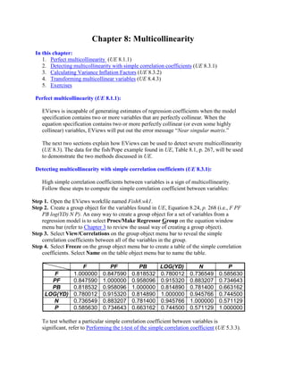
1. Chapter 8: Multicollinearity
In this chapter:
1. Perfect multicollinearity (UE 8.1.1)
2. Detecting multicollinearity with simple correlation coefficients (UE 8.3.1)
3. Calculating Variance Inflation Factors (UE 8.3.2)
4. Transforming multicollinear variables (UE 8.4.3)
5. Exercises
Perfect multicollinearity (UE 8.1.1):
EViews is incapable of generating estimates of regression coefficients when the model
specification contains two or more variables that are perfectly collinear. When the
equation specification contains two or more perfectly collinear (or even some highly
collinear) variables, EViews will put out the error message “Near singular matrix.”
The next two sections explain how EViews can be used to detect severe multicollinearity
(UE 8.3). The data for the fish/Pope example found in UE, Table 8.1, p. 267, will be used
to demonstrate the two methods discussed in UE.
Detecting multicollinearity with simple correlation coefficients (UE 8.3.1):
High simple correlation coefficients between variables is a sign of multicollinearity.
Follow these steps to compute the simple correlation coefficient between variables:
Step 1. Open the EViews workfile named Fish8.wk1.
Step 2. Create a group object for the variables found in UE, Equation 8.24, p. 268 (i.e., F PF
PB log(YD) N P). An easy way to create a group object for a set of variables from a
regression model is to select Procs/Make Regressor Group on the equation window
menu bar (refer to Chapter 3 to review the usual way of creating a group object).
Step 3. Select View/Correlations on the group object menu bar to reveal the simple
correlation coefficients between all of the variables in the group.
Step 4. Select Freeze on the group object menu bar to create a table of the simple correlation
coefficients. Select Name on the table object menu bar to name the table.
F PF PB LOG(YD) N P
F 1.000000 0.847590 0.818532 0.780012 0.736549 0.585630
PF 0.847590 1.000000 0.958096 0.915320 0.883207 0.734643
PB 0.818532 0.958096 1.000000 0.814890 0.781400 0.663162
LOG(YD) 0.780012 0.915320 0.814890 1.000000 0.945766 0.744500
N 0.736549 0.883207 0.781400 0.945766 1.000000 0.571129
P 0.585630 0.734643 0.663162 0.744500 0.571129 1.000000
To test whether a particular simple correlation coefficient between variables is
significant, refer to Performing the t-test of the simple correlation coefficient (UE 5.3.3).

2. Calculating Variance Inflation Factors (UE 8.3.2):
The procedure for calculating the Variance Inflation Factors (VIF's) for explanatory
variables in a regression model is explained in UE, p. 257. Use the following steps to
calculate the VIF for the PF explanatory variable in UE, Equation 8.24, p. 268:
Step 1. Open the EViews workfile named Fish8.wk1.
Step 2. Select Objects/New Object/Equation on the workfile menu bar, enter PF C PB
log(YD) N P in the Equation Specification: window, and click OK. Note the R2 =
0.976680.
Step 3. To save this regression, select Name on the equation window menu bar, enter EQPF
in the Name to identify object: window, and click OK.
Step 4. To calculate the VIF for the variable PF, write the equation: scalar VIFPF=1/(1-
EQPF.@R2) in the command window, and press Enter. The status line in the lower left
of the screen will display the phrase "VIFPF successfully created." A new variable
named VIFPF will appear in the workfile window.
Step 5. Double click on the VIFPF icon and the value for the Variance Inflation Factor for
the variable named VIFPF = 42.88… will be displayed on the status line (lower left of
the screen). The fact that VIFPF is significantly greater than 5 (i.e., the common rule of
thumb value stated in UE, p. 258), would suggest that PF exhibits severe
multicollinearity.
Step 6. Repeat Steps 2-5 to compute the Variance Inflation Factors for the rest of the
explanatory variables in UE, Equation 8.24, p. 268.
Transforming multicollinear variables (UE 8.4.3):
Variable transformations can be achieved by creating a new variable or by simply writing
the transformation in the Equation Specification: window in EViews. In many ways, the
latter is preferred because the equation output labels depict the transformation.
Otherwise, it is easy to forget what transformations have been made. The table below lists
the most common transformations used to rid a model of multicollinearity, along with the
EViews specification (EViews specification) to make it happen.
Function Name Description EViews specification
Linear combination Yt = β 0 + β 1(Xt + Zt ) Y C X+Z*
First difference Yt = β 0 + β 1(Xt - Xt-1) Y C d(X)
First difference of the logarithm Yt = β 0 + β 1(lnXt - lnXt-1) Y C dlog(X)
One-period % change (in decimal) Yt = β 0 + β 1[(Xt - Xt-1)/Xt ] Y C pch(X)
* no spaces in the X+Z variable designation.

3. Exercises:
8.
a.
b. Follow the steps outlined in Detecting multicollinearity with simple correlation
coefficients and Calculating Variance Inflation Factors to check for high
correlations and high VIF's in the implied regression model.
13. Follow the steps outlined in Detecting multicollinearity with simple correlation
coefficients and Calculating Variance Inflation Factors to check UE, Equation 8.25,
p. 269 for high correlations and high VIF's.
16.
f. Run the regressions for this problem using the Mine8.wf1 data set.
a) Refer to Chapter 5 for help with this part.
b) Refer to Detecting multicollinearity with simple correlation coefficients for
help with this part.
c) Refer to Transforming the multicollinear variables for help with this part.
d) Refer to Table with EViews specification for functional forms for help with
this part.