Download as PDF, PPTX
![Vectors Date/
Time
Series 1 Series 2
Vector 1 2:30:01 4.56 78.93
Vector 2 2:30:02 4.57 79.92
Vector 3 2:30:03 4.87 79.91
Vector 4 2:30:04 4.48 78.99
RDD[(ZonedDateTime, Vector)]
DateTime
Index
Vector for
Series 1
Vector for
Series 2
2:30:01 4.56 78.93
2:30:02 4.57 79.92
2:30:03 4.87 79.91
2:30:04 4.48 78.99
TimeSeriesRDD(
DateTimeIndex,
RDD[Vector]
)
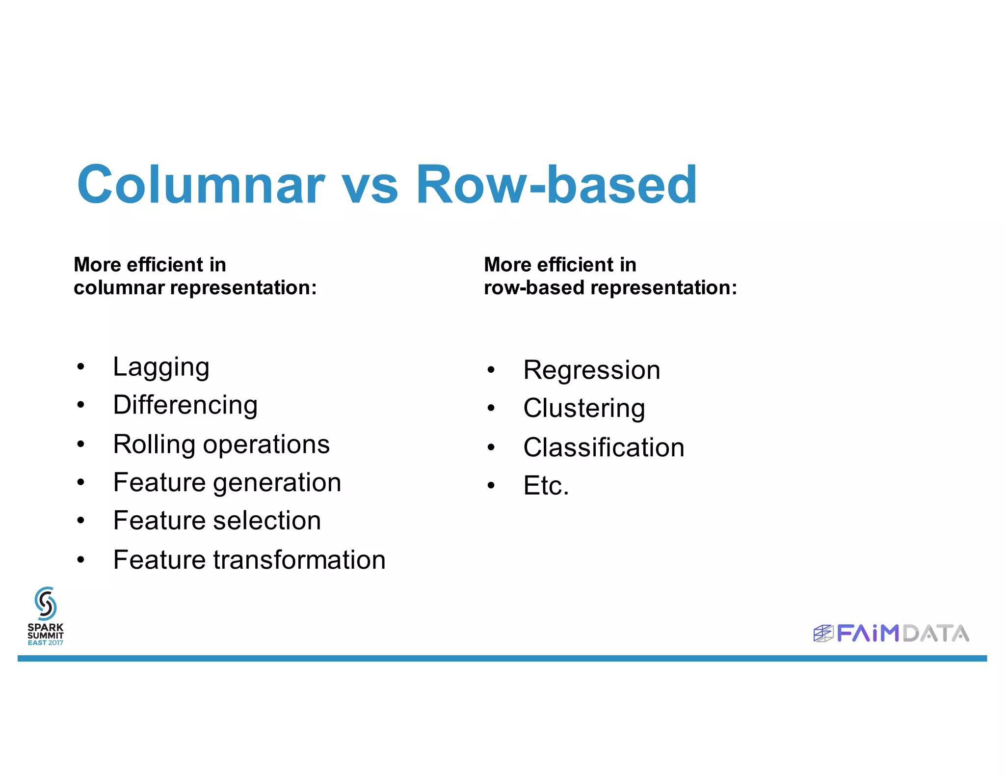
Columnar representation Row-based representation](https://image.slidesharecdn.com/2asimonouellette-170214185944/75/Time-Series-Analytics-with-Spark-Spark-Summit-East-talk-by-Simon-Ouellette-6-2048.jpg)
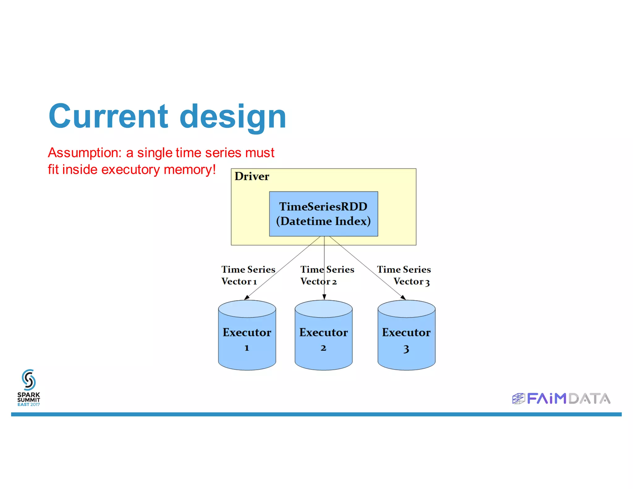
![Current design
Assumption: a single time series must
fit inside executory memory!
TimeSeriesRDD (
DatetimeIndex,
RDD[(K, Vector)]
)
IrregularDatetimeIndex (
Array[Long], // Other limitation: Scala arrays = 232 elements
java.time.ZoneId
)](https://image.slidesharecdn.com/2asimonouellette-170214185944/75/Time-Series-Analytics-with-Spark-Spark-Summit-East-talk-by-Simon-Ouellette-15-2048.jpg)
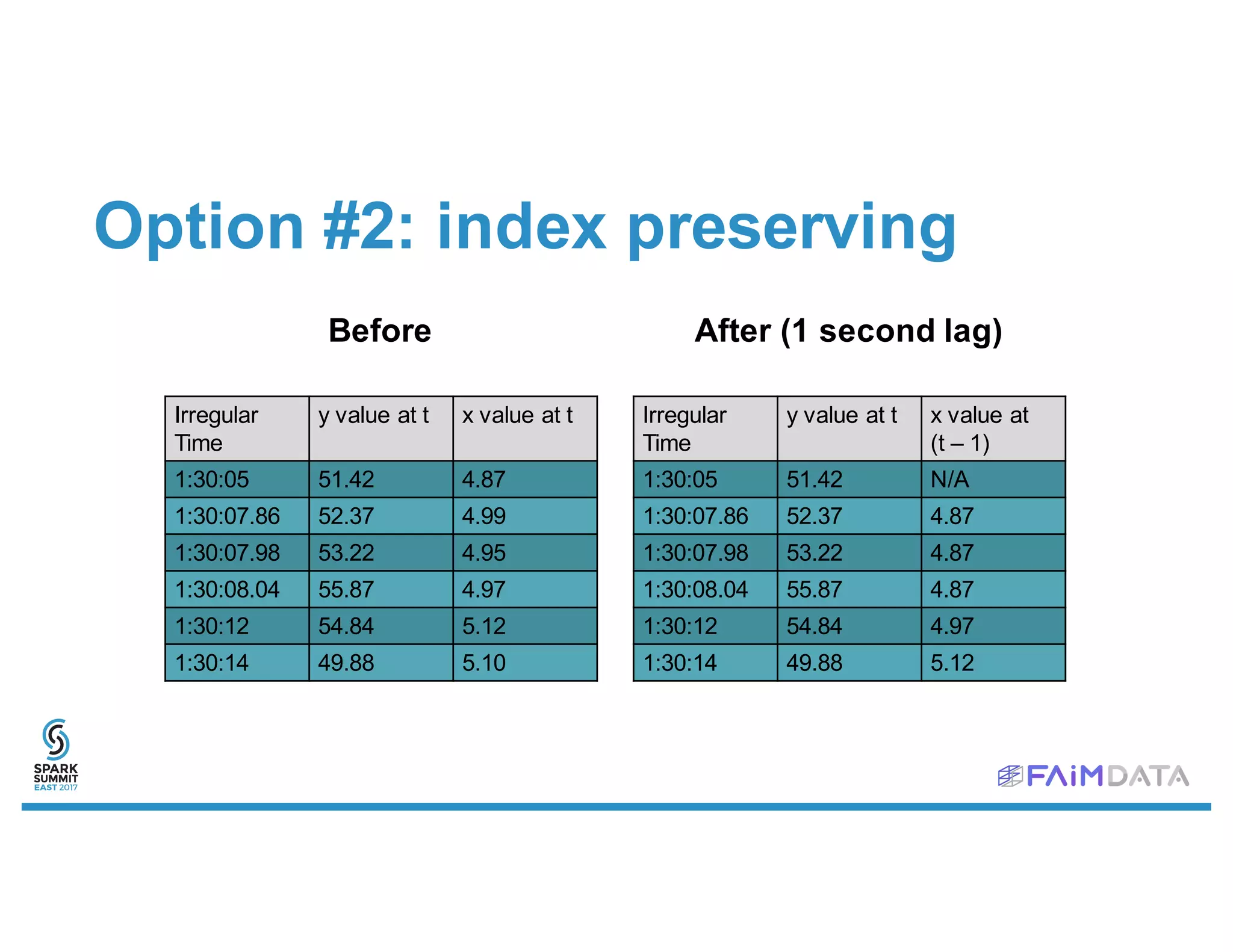
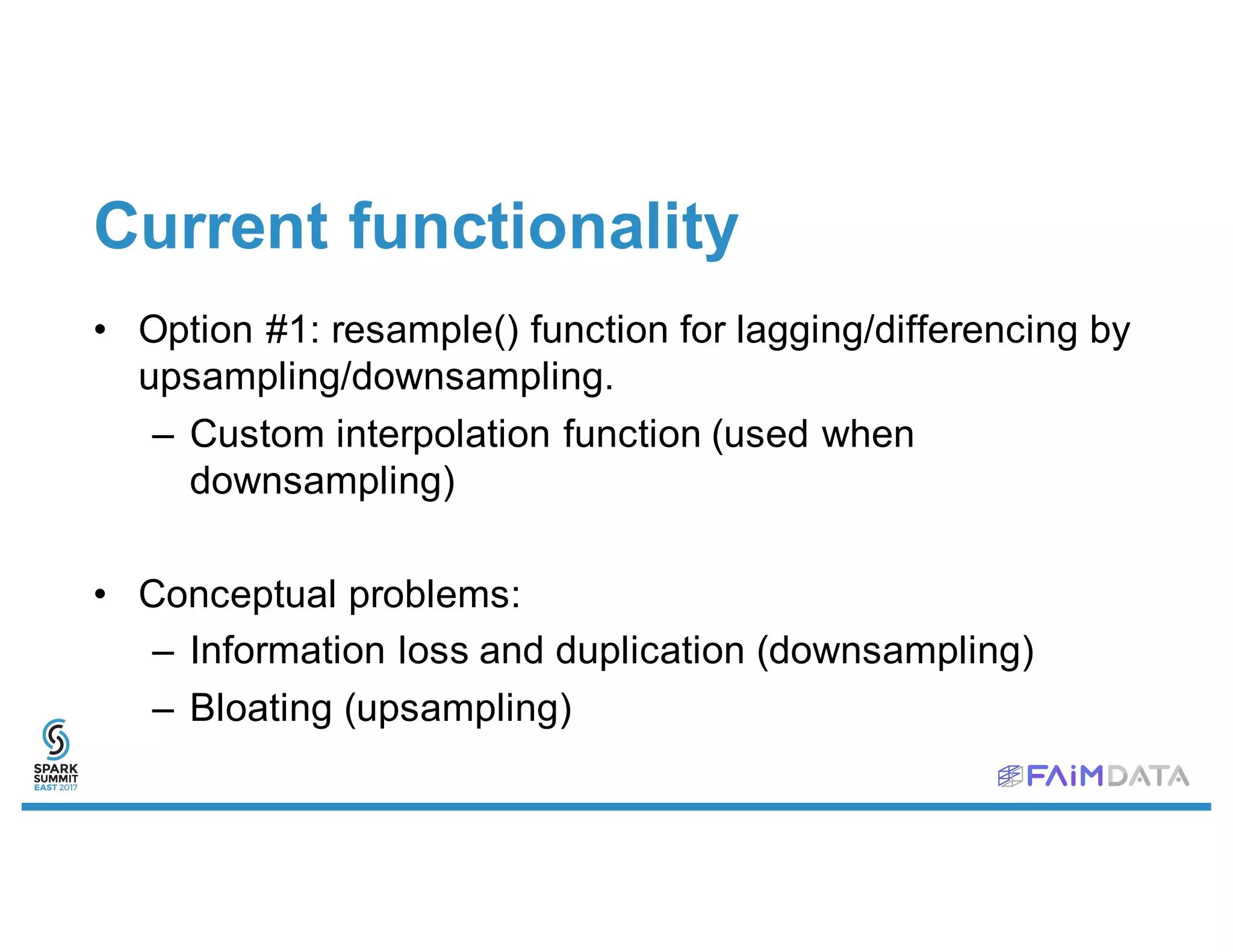
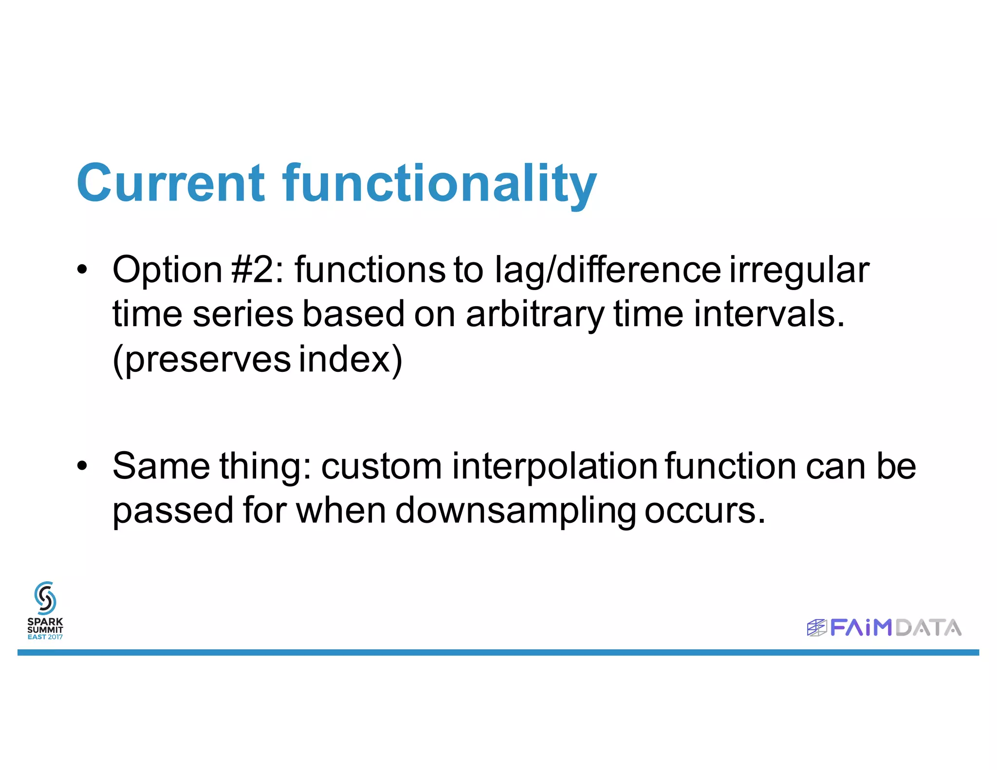
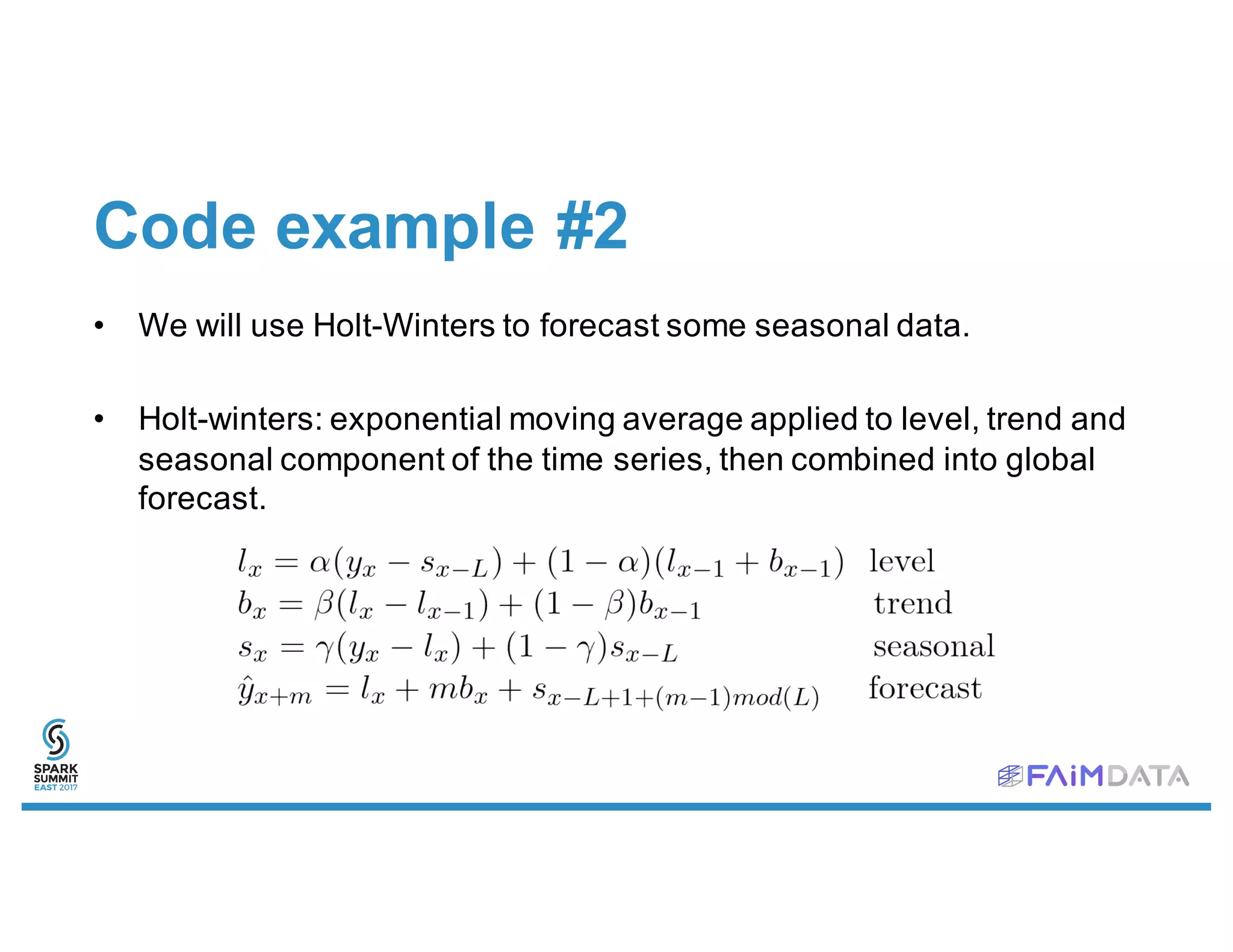
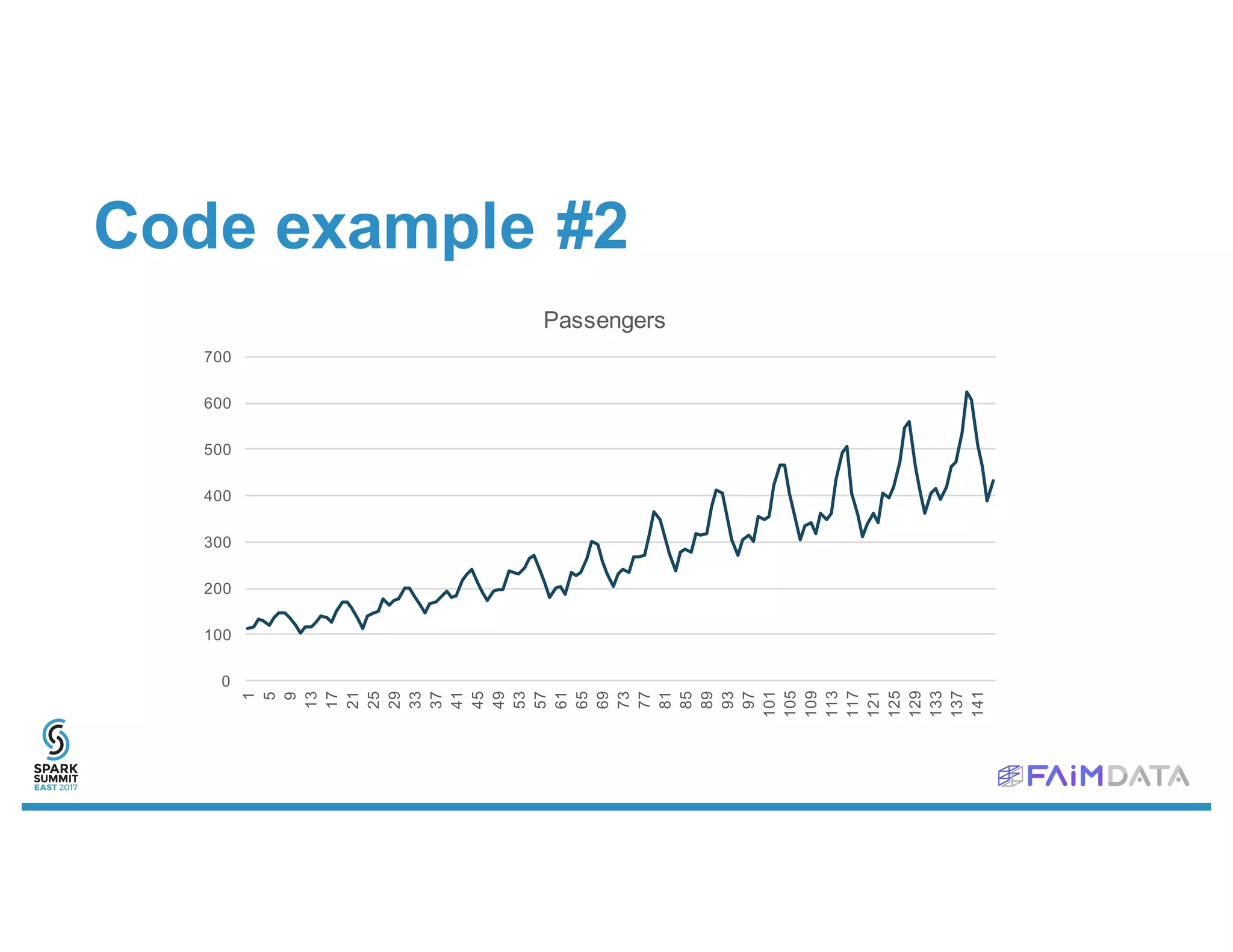
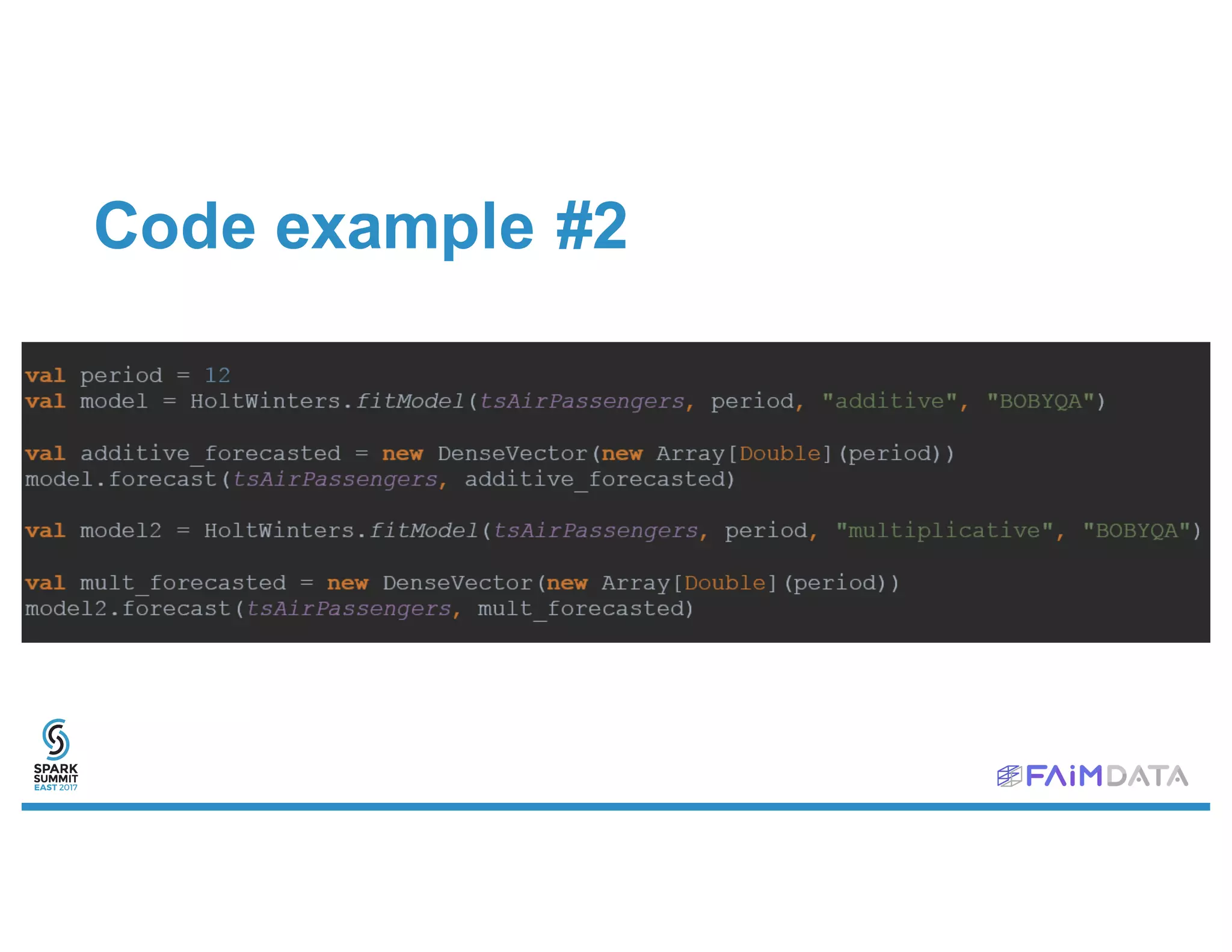
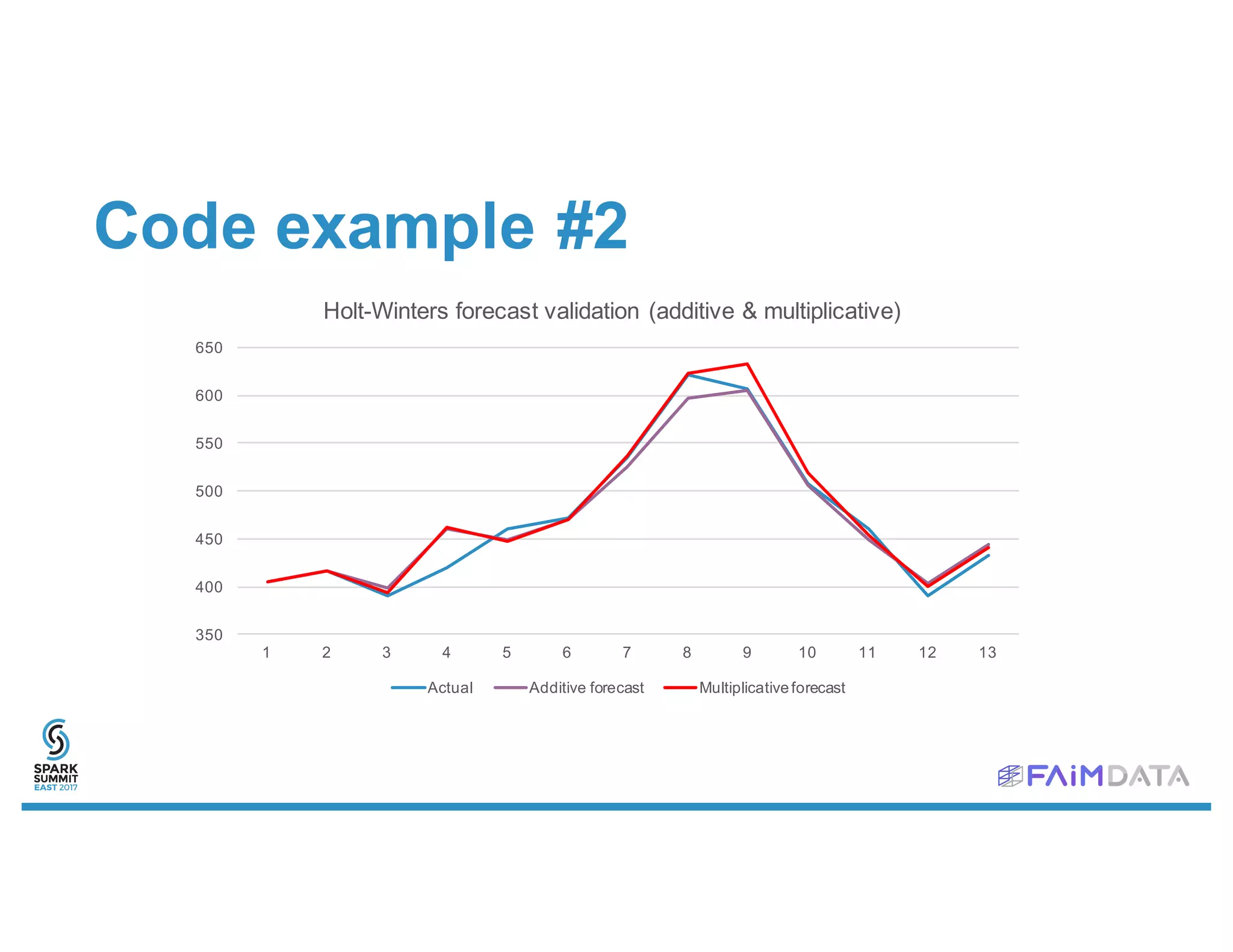

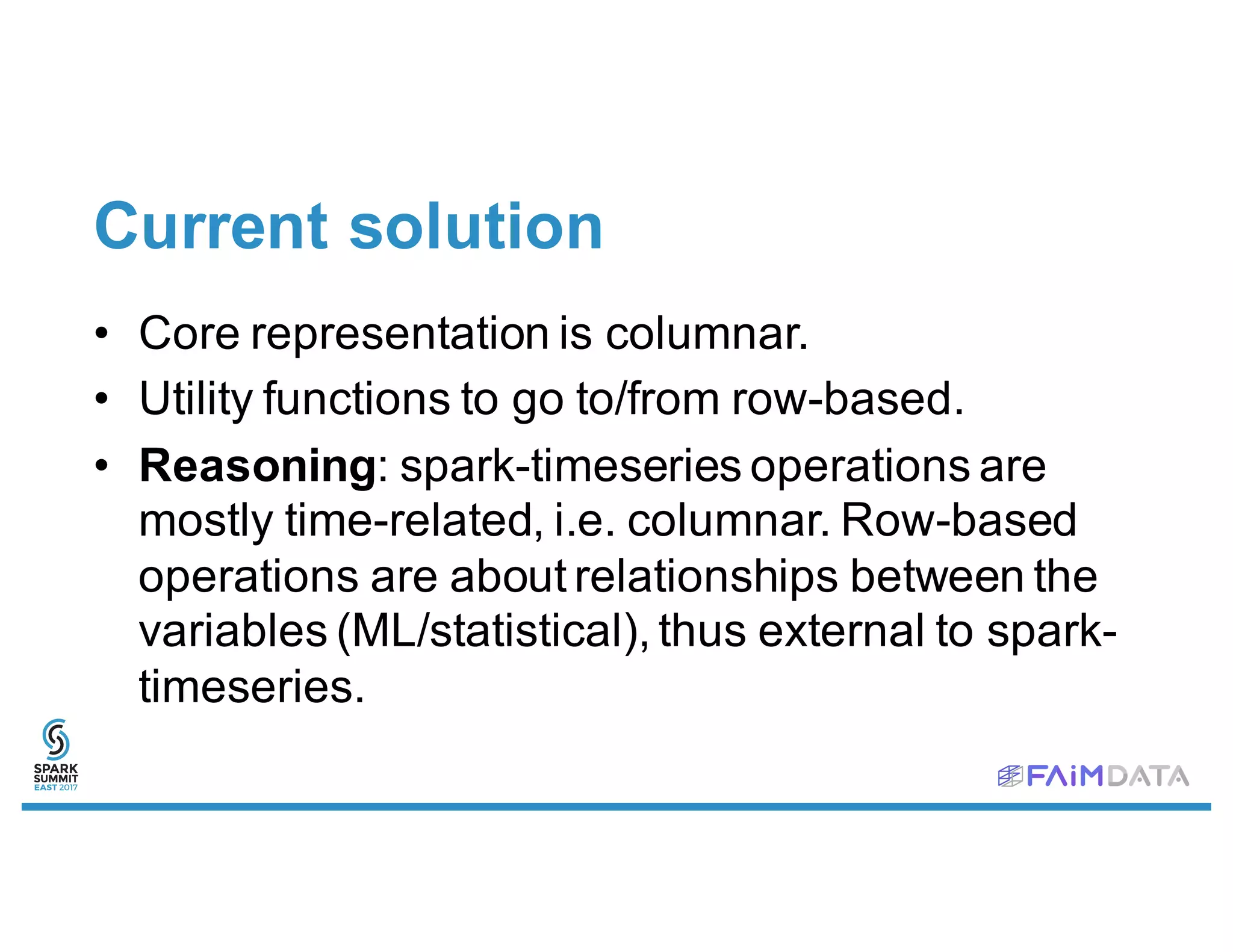
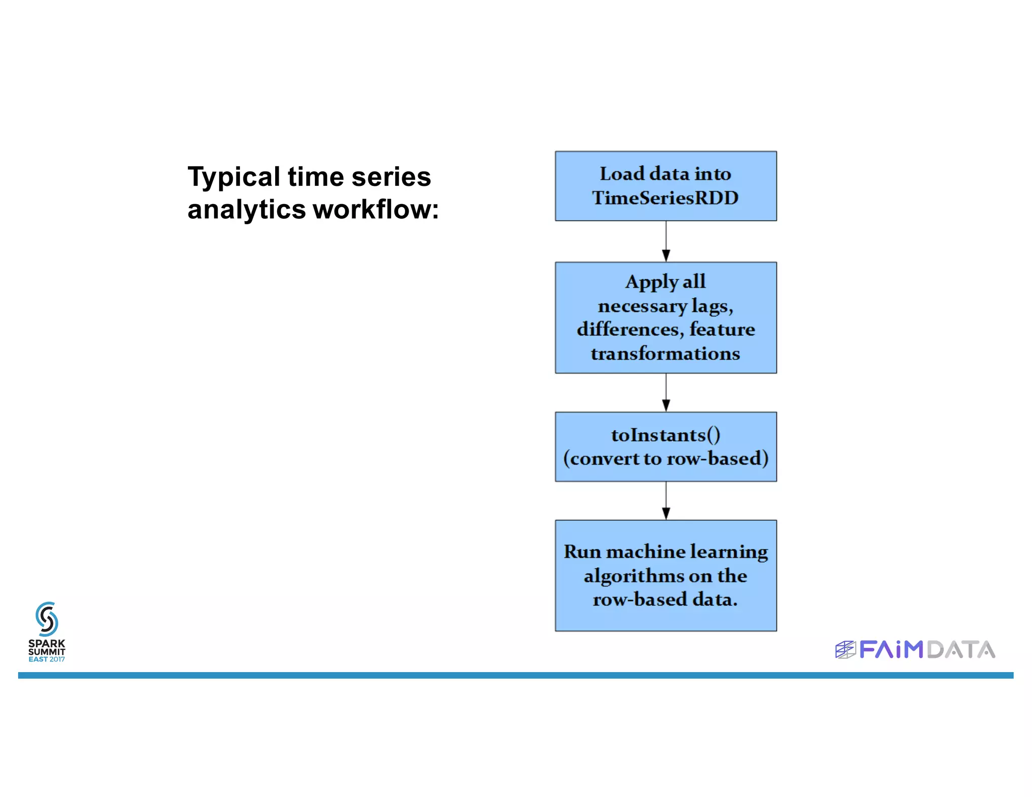
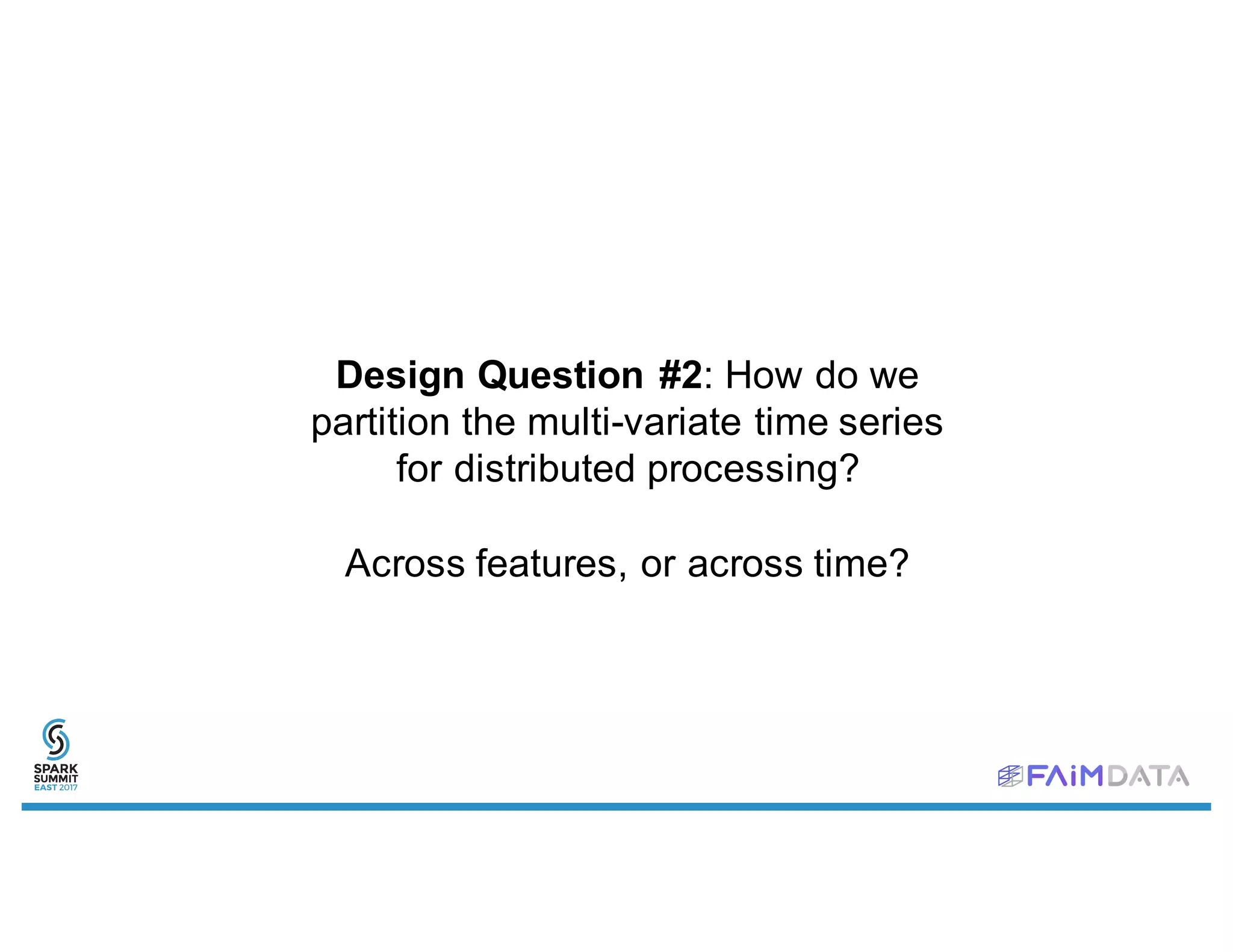
This document provides an overview of spark-timeseries, an open source time series library for Apache Spark. It discusses the library's design choices around representing multivariate time series data, partitioning time series data for distributed processing, and handling operations like lagging and differencing on irregular time series data. It also presents examples of using the library to test for stationarity, generate lagged features, and perform Holt-Winters forecasting on seasonal passenger data.


![Introduction to Pandas and Time Series Analysis [PyCon DE]](https://cdn.slidesharecdn.com/ss_thumbnails/introductiontopandasandtimeseriesanalysispyconde-170617163724-thumbnail.jpg?width=640&height=640&fit=bounds)


![Introduction to Data Analtics with Pandas [PyCon Cz]](https://cdn.slidesharecdn.com/ss_thumbnails/introductiontodataanalticswithpandaspyconcz-170617163446-thumbnail.jpg?width=640&height=640&fit=bounds)

![Introduction to Pandas and Time Series Analysis [Budapest BI Forum]](https://cdn.slidesharecdn.com/ss_thumbnails/introductiontopandasandtimeseriesanalysis-170617163829-thumbnail.jpg?width=640&height=640&fit=bounds)


![[DSC Europe 25] Dobrica Cosic - Savings by the Second: How Dynamic Pricing an...](https://cdn.slidesharecdn.com/ss_thumbnails/znp09f3smtqz3w2sq6wn-1-dobrica-cosic-savings-by-the-second-how-dynamic-pricing-and-smart-data-are-bu-251208151905-26e6f41e-thumbnail.jpg?width=640&height=640&fit=bounds)


![[DSC Europe 25] Marko Krstic - Understanding the AI Threat Landscape - Risks,...](https://cdn.slidesharecdn.com/ss_thumbnails/tiyim1ins5jvbrvzpzla-2-251209104645-c69d3553-thumbnail.jpg?width=640&height=640&fit=bounds)
![[DSC Europe 25] Branko Dzakula - From Defense to Attack: How AI Redefines Cyb...](https://cdn.slidesharecdn.com/ss_thumbnails/80bdzdxpr3ky2g0qvyk9-8-251211083048-ce5fc1ee-thumbnail.jpg?width=640&height=640&fit=bounds)
![[DSC Europe 25] Vladimir Jelic - The AI-Driven Security Shift From Reactive D...](https://cdn.slidesharecdn.com/ss_thumbnails/6g5gj25mtjwayniqem1t-6-251209104645-7a5a5fc6-thumbnail.jpg?width=640&height=640&fit=bounds)


![[DSC Europe 25] Dragana Ilic - AI for Big Data in Astronomy.pptx](https://cdn.slidesharecdn.com/ss_thumbnails/8palya86qaatvjhva1ms-2-dragana-ilic-ai-ilic-251208151906-652b819c-thumbnail.jpg?width=640&height=640&fit=bounds)
![[DSC Europe 25] Dusan Pavlov - There Is No Spoon: Inferring Vision from Neura...](https://cdn.slidesharecdn.com/ss_thumbnails/wg0v1umoqjm4nnbd3p0v-there-is-no-spoon-251205085715-6d81d6c5-thumbnail.jpg?width=640&height=640&fit=bounds)

![[DSC Europe 25] Imai Jen-La Plante - The New Generation: AI and the Future of...](https://cdn.slidesharecdn.com/ss_thumbnails/kxi8t2l5rggivgcenyba-1-jenlaplante-dsc-251208152532-d1e076c2-thumbnail.jpg?width=640&height=640&fit=bounds)

![[DSC Europe 25] Dragan Vucic - Building the Learning Organization - How AI Tr...](https://cdn.slidesharecdn.com/ss_thumbnails/8brigo2sbu6qur6gxrra-7-251205085715-6ae07d24-thumbnail.jpg?width=640&height=640&fit=bounds)
![[DSC Europe 25] Marija Vlajkovic & Andrea Radonjanin - Integration of AI tool...](https://cdn.slidesharecdn.com/ss_thumbnails/qf1jrglttoc3bm8s3aop-final-integration-of-ai-tools-251208151905-394f3a6a-thumbnail.jpg?width=640&height=640&fit=bounds)
![[DSC Europe 25] Sara Polak - The Ancient Operating System: What Archaeology T...](https://cdn.slidesharecdn.com/ss_thumbnails/3vch2p6tttdnwhsgazoz-3-sara-polak-smart-cities-251208152532-64404202-thumbnail.jpg?width=640&height=640&fit=bounds)
