The document provides solutions to multiple problems involving calculating Thevenin and Norton equivalents for various circuits. Some key steps include:
1) Removing independent sources and determining the equivalent voltage (VOC) and resistance (RTH) between terminals.
2) Finding the short circuit current (ISC) to calculate RTH if dependent sources are present.
3) Drawing the equivalent Thevenin or Norton circuit and using it to solve for desired values like current through a load resistor.
4) For maximum power transfer problems, equating RTH to the load resistance and calculating the maximum power.
The superposition theorem allows analysts to determine the voltage across or current through an element in a linear, bilateral circuit containing multiple sources. It states that the response of such a circuit to multiple sources is equal to the sum of the responses to each source acting alone. To apply the theorem, each independent source is solved for separately while other sources are removed by shorting or opening. Dependent sources are left intact. The procedure is demonstrated through examples solving for currents using superposition in circuits with independent and dependent sources.
The document discusses the structure of the sodium D line spectrum. It explains that sodium has 11 electrons with one valence electron in the third shell. The state of the sodium atom is defined by the state of this valence electron. It also discusses that alkali metal atoms like sodium have one valence electron and diagrams the energy levels of sodium as the P, S, D levels with J values. It introduces the concept of screening constants which account for the number of closed shell electrons that screen the nucleus from the valence electron. Finally, it discusses the quantum defect value which depends on the orbital quantum number and is positive for sodium.
The document describes the fixed-bias configuration for an n-channel JFET. It provides equations that relate the input and output quantities for JFETs and shows how to analyze the fixed-bias configuration using both a mathematical and graphical approach. The key points are:
- The fixed-bias configuration has a fixed gate-to-source voltage VGS determined by the fixed DC supply VGG.
- Shockley's equation relates the drain current ID to VGS and can be plotted as a curve.
- For analysis, a vertical line is drawn at the fixed VGS and the point where it intersects the curve determines the operating point (IDQ, VGSQ).
- Both mathematical calculations
This document describes an experiment on negative feedback amplifiers using BJT transistors. The objectives are to study the influence of negative feedback, examine feedback amplifier properties experimentally, and determine input/output impedance, gain, and bandwidth with and without feedback. The procedures measure these characteristics for common feedback configurations - voltage series, current series, current shunt, and voltage shunt. Input/output impedance is measured by varying a test resistance until output amplitude is halved. Gain is calculated from input and output voltages. Bandwidth is found by varying frequency until output amplitude is 0.707 times maximum. The gain-bandwidth product is also calculated.
1) Bipolar junction transistors (BJTs) are three-terminal semiconductor devices with an emitter, collector, and base. There are npn and pnp types depending on the doping of each region.
2) In BJTs, the base current controls the collector and emitter currents. A small change in base current results in a larger change in collector and emitter currents. The relationship between these currents is characterized by parameters like beta and alpha.
3) BJT operation depends on the biasing of the base-emitter and collector-base junctions. In cutoff, both junctions are reverse biased and little current flows. In active operation, the base-emitter junction is
It covers all the Maxwell's Equation for Point form(differential form) and integral form. It also covers Gauss Law for Electric Field, Gauss law for magnetic field, Faraday's Law and Ampere Maxwell law. It also covers the reason why Gauss Laws are also known as Maxwell's Equation.
Oscillator is a mechanical or electronic device works on the principle of oscillation i.e. a periodic fluctuation between two things based on changes in energy. It is of two types; linear oscillators and non linear oscillators. The wave shape and amplitude are determined by the design of the oscillator circuit and choice of component values.
The document describes a two port network and provides information about various parameter representations of two port networks, including:
- Z parameters define the input and transfer impedances between the two ports.
- Y parameters define the input and transfer admittances between the two ports.
- Transmission parameters (A,B,C,D) define relationships between voltages and currents at the two ports.
- Hybrid parameters also define relationships between voltages and currents at the two ports.
Examples are provided to demonstrate calculating the parameter representations for given two port networks. Additionally, the document discusses how modifying a two port network impacts its parameter representations.
Eigenvalues and eigenfunctions are key concepts in linear algebra. An eigenfunction is a function that when operated on by a linear operator produces a constant multiplied version of itself. The constant is the corresponding eigenvalue. Eigenvalues are the solutions to the characteristic polynomial of the linear operator. Eigenfunctions are not unique as any constant multiple of an eigenfunction is also an eigenfunction with the same eigenvalue. The spectrum of an operator is the set of all its eigenvalues.
This laboratory manual describes an experiment to verify Ohm's law. The experiment involves measuring the current and voltage across resistors with values of 1kΩ, 10kΩ, and 100kΩ as the supply voltage is varied. Ohm's law states that voltage is equal to current times resistance. The results are plotted on a graph of current versus voltage to verify the linear relationship predicted by Ohm's law and observe how the slope changes with different resistances.
A three-phase system uses three sinusoidal voltages that are 120 degrees out of phase to provide constant power output. A balanced three-phase system can be analyzed using a single-phase equivalent circuit. Power in a three-phase system is measured using three wattmeters connected in a Y configuration for a Y-connected load or two wattmeters connected between line voltages for a three-wire system. The total power is the sum of the wattmeter readings.
Fourier series can be used to represent periodic and discontinuous functions. The document discusses:
1. The Fourier series expansion of a sawtooth wave, showing how additional terms improve the accuracy of the representation.
2. How Fourier series are well-suited to represent periodic functions over intervals like [0,2π] since the basis functions are also periodic.
3. An example of using Fourier series to analyze a square wave, finding the coefficients for its expansion in terms of sines and cosines.
This document provides a summary of key concepts related to electromagnetic induction and Maxwell's equations:
1) Faraday's law describes how a changing magnetic flux induces an electromotive force (emf). A changing magnetic field can also induce an electric field.
2) Maxwell proposed adding a "displacement current" term to Ampere's law to account for time-varying electric fields. This completes the theory to show that changing electric fields generate magnetic fields.
3) Maxwell's full set of equations symmetrically relate the electric and magnetic fields and show they are interdependent. In the absence of charges, the equations imply a relationship between electromagnetic phenomena and the speed of light.
This document section describes alternating current (AC) circuits containing a single circuit element: resistor, inductor, or capacitor, connected to an AC voltage source. For a resistive circuit, the current and voltage are in phase. For an inductive circuit, the current lags the voltage by 90 degrees. For a capacitive circuit, the current leads the voltage by 90 degrees. The document defines important concepts such as reactance, impedance, and phasor diagrams for analyzing AC circuits.
This document defines and discusses orthogonal vectors, unit/normalized vectors, orthogonal and orthonormal sets of vectors, the relationship between independence and orthogonality of vectors, vector projections, and the Grahm-Schmidt orthogonalization process. Specifically, it states that two vectors are orthogonal if their dot product is zero, an orthogonal set is linearly independent, the difference between a vector and its projection onto another vector is orthogonal to that vector, and the Grahm-Schmidt process constructs new orthogonal vectors.
The document discusses three-phase circuits and provides information on:
- The advantages of three-phase supply systems such as higher efficiency of power transfer and smoother load characteristics.
- Key concepts like phase sequence, balanced/unbalanced supply and load, and the relationships between line and phase voltages and currents.
- How to calculate power in a balanced three-phase system and use two wattmeters to measure total power and power factor.
The document describes calculating currents in a star-connected load using symmetrical components. It finds:
Ia1 = 13.8461 - 0.0000i
Ia2 = 2.3077 + 1.3324i
Ia = 16.1539 + 1.3323i
Vn = 38.4614 -13.3234i
It also solves another example finding line currents Ia, Ib, Ic for a delta-connected load from line voltages using symmetrical components. Relations between symmetrical components of line and phase quantities are also examined.
This document describes a study that designed a fuzzy logic controller for a boost DC-DC converter using MATLAB/Simulink software. The objective was to develop a fuzzy logic algorithm to control the output voltage of the boost converter in steady state conditions. Simulation results showed that the fuzzy logic controller was able to maintain the output voltage with no overshoot, unlike the open loop converter which had 80% overshoot. In conclusion, the fuzzy logic controller improved the dynamic performance and stability of the boost converter compared to an open loop design.
The document contains 6 problems analyzing diode circuits using ideal diode and constant voltage drop models:
1. Finds the Q-point for a single diode circuit using a load line.
2. Calculates the Q-point for two diode circuits using ideal and constant voltage drop models.
3. Finds the Q-point for a diode circuit and compares ideal diode and constant voltage drop models.
4. Calculates voltages and currents for 4 diode circuits using ideal and constant voltage drop models.
5. Repeats problem 4 with increased resistor values.
6. Finds the Q-points for 3 diodes in different configurations using the ideal diode model.
This document discusses three-phase AC circuits. It begins by describing some disadvantages of single-phase systems, such as induction motors not being self-starting. Three-phase systems are then introduced as having advantages like constant power transmission. Balanced three-phase systems are defined as having three voltage sources 120 degrees out of phase. The document covers the different connection types between a three-phase source and load, such as wye-wye, and provides equations to calculate line and phase voltages and currents.
Ch5 lecture slides Chenming Hu Device for ICChenming Hu
This document summarizes key concepts about MOS capacitors including:
1) The structure and operation of an MOS capacitor including accumulation, depletion, and inversion regions depending on the gate voltage Vg relative to the flat-band voltage Vfb and threshold voltage Vt.
2) Equations relating surface potential φs, depletion width Wdep, oxide capacitance Cox, and inversion charge Qinv to the applied gate voltage Vg.
3) Sources of threshold voltage Vt variation including body doping, oxide thickness Tox, and fixed oxide charge Qox.
4) Effects of poly-silicon gate depletion on the effective oxide thickness and inversion charge Qinv.
The document discusses three-phase circuits and their analysis. It covers balanced and unbalanced three-phase configurations, power in balanced systems, and analyzing unbalanced systems using PSpice. The objectives are to understand different three-phase connections, distinguish balanced and unbalanced circuits, calculate power in balanced systems, analyze unbalanced systems, and apply the concepts to measurement and residential wiring. Key points covered include wye-wye, wye-delta, delta-delta, and delta-wye connections for both sources and loads.
1) Gauss's law relates the electric flux through a closed surface to the enclosed electric charge. It can be used to calculate the electric field from a charge distribution if symmetry is present.
2) The document explores if there is an inverse expression that can locally calculate the charge density from the electric field. It examines calculating the electric flux through an infinitesimally small volume element.
3) By taking the sum of the fluxes through all sides of the small volume element and equating it to the enclosed charge, it derives that the divergence of the electric field equals the charge density divided by the permittivity of free space. This allows locally calculating the charge density from the electric field.
The document defines a tie-set as a set of branches that form a closed path or loop in a graph containing one link and remaining twigs. A tie-set is also known as a fundamental circuit or f-circuit. The number of tie-sets or loops in a graph equals the number of links. A tie-set matrix describes how branches constitute loops in a graph using an ordered list and reference direction for each loop. Examples of tie-set matrices for different trees are provided.
Engineering review on AC circuit steady state analysis.
Presentation lecture for energy engineering class.
Course: MS in Renewable Energy Engineering, Oregon institute of technology
This document discusses the Gamma and Beta functions. It defines them using improper definite integrals and notes they are special transcendental functions. The Gamma function was introduced by Euler and both functions have applications in areas like number theory and physics. The document provides properties of each function and examples of evaluating integrals using their definitions and relations.
This document contains the answers to a 30 question multiple choice network theory test taken on June 10, 2017. The answers are provided in a numbered list from 1 to 30 without the corresponding questions. An answer key for the test is also included which provides the answers. The document aims to provide the answers to a network theory test for a student.
This document provides an introduction to electrostatics and discusses electric charges, atomic structure, early theories of electricity from Thales and Franklin, conduction and insulation, Coulomb's law for electrostatic force between two charges, and examples of calculating electrostatic force and potential. It defines key terms like electrostatics, charge, proton, electron, conductor, insulator, and Coulomb's law. Diagrams and examples throughout illustrate electrostatic concepts and their applications.
SolutionsPlease see answer in bold letters.Note pi = 3.14.docxrafbolet0
Solution
s:
Please see answer in bold letters.
Note pi = 3.1415….
1. The voltage across a 15Ω is as indicated. Find the sinusoidal expression for the current. In addition, sketch the v and i waveform on the same axis.
Note: For the graph of a and b please see attached jpg photo with filename 1ab.jpg and for c and d please see attached photo with filename 1cd.jpg.
a. 15sin20t
v= 15sin20t
By ohms law,
i = v/r
i = 15sin20t / 15
i = sin20t A
Computation of period for graphing:
v= 15sin20t
i = sin20t
w = 20 = 2pi*f
f = 3.183 Hz
Period =1/f = 0.314 seconds
b. 300sin (377t+20)
v = 300sin (377t+20)
i = 300sin (377t+20) /15
i = 20 sin (377t+20) A
Computation of period for graphing:
v = 300sin (377t+20)
i = 20 sin (377t+20)
w = 377 = 2pi*f
f = 60 Hz
Period = 1/60 = 0.017 seconds
shift to the left by:
2pi/0.017 = (20/180*pi)/x
x = 9.44x10⁻⁴ seconds
c. 60cos (wt+10)
v = 60cos (wt+10)
i = 60cos (wt+10)/15
i = 4cos (wt+10) A
Computation of period for graphing:
let’s denote the period as w sifted to the left by:
10/180*pi = pi/18
d. -45sin (wt+45)
v = -45sin (wt+45)
i = -45sin (wt+45) / 15
i = -3 sin (wt+45) A
Computation of period for graphing:
let’s denote the period as w sifted to the left by:
45/180 * pi = 1/4*pi
2. Determine the inductive reactance (in ohms) of a 5mH coil for
a. dc
Note at dc, frequency (f) = 0
Formula: XL = 2*pi*fL
XL = 2*pi* (0) (5m)
XL = 0 Ω
b. 60 Hz
Formula: XL = 2*pi*fL
XL = 2 (60) (5m)
XL = 1.885 Ω
c. 4kHz
Formula: XL = 2*pi*fL
XL = = 2*pi* (4k)(5m)
XL = 125.664 Ω
d. 1.2 MHz
Formula: XL = 2*pi*fL
XL = 2*pi* (1.2 M) (5m)
XL = 37.7 kΩ
3. Determine the frequency at which a 10 mH inductance has the following inductive reactance.
a. XL = 10 Ω
Formula: XL = 2*pi*fL
Express in terms in f:
f = XL/2 pi*L
f = 10 / (2pi*10m)
f = 159.155 Hz
b. XL = 4 kΩ
f = XL/2pi*L
f = 4k / (2pi*10m)
f = 63.662 kHz
c. XL = 12 kΩ
f = XL/2piL
f = 12k / (2pi*10m)
f = 190.99 kHz
d. XL = 0.5 kΩ
f = XL/2piL
f = 0.5k / (2pi*10m)
f = 7.958 kHz
4. Determine the frequency at which a 1.3uF capacitor has the following capacitive reactance.
a. 10 Ω
Formula: XC = 1/ (2pifC)
Expressing in terms of f:
f = 1/ (2pi*XC*C)
f = 1/ (2pi*10*1.3u)
f = 12.243 kΩ
b. 1.2 kΩ
f = 1/ (2pi*XC*C)
f = 1/ (2pi*1.2k*1.3u)
f = 102.022 Ω
c. 0.1 Ω
f = 1/ (2pi*XC*C)
f = 1/ (2pi*0.1*1.3u)
f = 1.224 MΩ
d. 2000 Ω
f = 1/ (2pi*XC*C)
f = 1/ (2pi*2000*1.3u)
f = 61.213 Ω
5. For the following pairs of voltage and current, indicate whether the element is a capacitor, an inductor and a capacitor, an inductor, or a resistor and find the value of C, L, or R if insufficient data are given.
a. v = 55 sin (377t + 50)
i = 11 sin (377t -40)
Element is inductor
In this case voltage leads current (ELI) by exactly 90 degrees so that means the circuit is inductive and the element is inductor.
XL = 55/11 = 5 Ω
we know the w=2pif so
w= 377=2pif
f= 60 Hz
To compute for th.
Solutions manual for fitzgerald and kingsleys electric machinery 7th edition ...crush424
Full clear download (no error formatting) at : https://goo.gl/XxyFcE
electric machinery 7th edition pdf
electric machinery fitzgerald 7th edition solution
fitzgerald & kingsley's electric machinery 7th edition umans pdf
electric machinery fitzgerald 7th edition solution pdf
electric machinery fitzgerald 5th edition pdf
electric machinery fitzgerald 6th edition solution
electric machinery fitzgerald 6th edition download
fitzgerald & kingsley’s electric machinery 7th pdf
This document contains a sample multiple choice question (MCQ) exam for electronics and communication engineering. It includes 15 sample questions related to basic electrical concepts such as current, voltage, resistance, capacitance and circuits. It also provides the solutions and explanations for each question. The document is from a book titled "GATE EC by RK Kanodia" which is intended to help students prepare for the graduate aptitude test in engineering exam for electronics and communication.
This document contains solved problems related to electronic devices such as transistors, diodes, and semiconductors. It includes 9 problems solved step-by-step relating to semiconductor properties and diode circuits. The problems calculate values such as intrinsic field, resistivity, drift velocity, current, activation voltages, and diode currents in various circuits using given component values and semiconductor parameters.
This document describes a study measuring the fraction of J/ψ mesons originating from Υ(1P), Υ(2P), and Υ(3P) decays as a function of pT(J/ψ) using data collected by the LHCb experiment at center-of-mass energies of 7 and 8 TeV. The analysis involves determining yields of J/ψ mesons and yields from Υ decays to J/ψ in different pT bins. Monte Carlo simulations are used to calculate efficiencies and compare data distributions. Results include improved precision on previous LHCb measurements of these fractions and a measurement of the Υ1(3P) mass.
The document advertises free solution manuals and textbooks for many university-level books. It states that the solution manuals contain fully solved and clearly explained solutions to all the exercises in the textbooks. It encourages visiting the website to download the files for free.
Electic circuits fundamentals thomas floyd, david buchla 8th edition명중 김
This document provides solutions to end-of-chapter problems from a textbook on quantities and units. The solutions cover topics in scientific notation, engineering notation, metric prefixes, and unit conversions. Specifically, it provides step-by-step workings and answers to over two dozen problems across multiple sections of Chapter 1.
This document contains review questions and practice problems related to transistor (BJT) circuit analysis. The review questions cover topics like current gains, transistor biasing, I-V characteristics, and transistor operation. The practice problems involve calculating operating points, currents, and voltages in common emitter amplifier circuits using transistor parameters like current gain β and bias voltages. Solving the problems requires applying concepts like Kirchhoff's laws and transistor modeling.
Linear circuit analysis - solution manuel (R. A. DeCarlo and P. Lin) (z-lib.o...Ansal Valappil
This document provides solutions to multiple physics problems related to electricity and circuits. Solution 1.1 calculates the net charge on a sphere with 10^13 electrons. Solution 1.2 calculates the number of atoms and total charge in a sample of copper. Solution 1.3 calculates current flowing based on the charge and time.
The document contains 14 exercise problems related to analyzing bias points of transistors. Problem 1 asks to find the bias point of a transistor with β = 100 and VA → ∞. Problem 4 asks to find the bias point of a transistor with β = 200 and VA → ∞. Problem 6 asks to find the bias point of a transistor, determine the Thevenin equivalent of the voltage divider, and that the base voltage must be large enough to forward bias the BE junction.
Solutions manual for cmos digital integrated circuits analysis and design 4th...Blitzer567
People also search:
cmos digital integrated circuits 4th edition pdf
cmos digital integrated circuits analysis & design 4th edition
cmos digital integrated circuits analysis and design 3rd edition solution manual
analysis and design of digital integrated circuits pdf
cmos digital circuit design
cmos digital integrated circuits a first course pdf
digital integrated circuit design
digital integrated circuits analysis and design ayers solution manual
Cmos digital integrated circuits analysis and design 4th edition kang solutio...vem2001
CMOS Digital Integrated Circuits Analysis and Design 4th Edition Kang Solutions Manual
Download:https://goo.gl/n2KuTT
cmos digital integrated circuits 4th edition pdf
cmos digital integrated circuits analysis & design 4th edition
cmos digital integrated circuits analysis and design 3rd edition solution manual
cmos kang solutions chapter 6
cmos digital circuits
analysis and design of digital integrated circuits hodges pdf free download
digital integrated circuits pdf
analysis and design of digital integrated circuits pdf
Grid Converters for Photovoltaic and Wind Power Systems - 2010 - Teodorescu -...gulie
This document summarizes space vector transformations of three-phase systems. It discusses symmetrical components analysis in the frequency and time domains, which allows decomposition of an unbalanced three-phase system into positive, negative, and zero sequence components. It also describes Clarke's transformation to a stationary αβ0 reference frame, which defines three independent real components from the complex positive and negative sequence components.
The document summarizes a presentation on power management in DC microgrids. It outlines the presenter's coursework credits and GPA. It then introduces the importance of ensuring dynamic stability in microgrids to achieve safe and reliable performance. The presentation covers various converter topologies used in DC microgrids, including the KY-boost, Sepic, and Cuk converters. State-space models and analyses of these converters are provided through equations and frequency response plots.
This document contains solutions to chapter 14 problems from the 7th edition of Engineering Circuit Analysis. It includes multiple pages with solutions to circuit analysis problems involving complex frequencies. The solutions provide the complex frequency (s) associated with different circuit variables like voltage and current. Key information includes identifying the complex frequency of signals, calculating impedances of circuit elements, and determining voltages and currents using complex frequency analysis.
This document contains 12 solutions to physics problems related to dynamics and kinematics. The solutions calculate things like work, acceleration, forces, velocities, distances, and times using concepts like Newton's laws of motion, kinematics equations, coefficients of friction, and inclines. Equations are set up and solved to find the requested unknown variables.
Redefining brain tumor segmentation: a cutting-edge convolutional neural netw...IJECEIAES
Medical image analysis has witnessed significant advancements with deep learning techniques. In the domain of brain tumor segmentation, the ability to
precisely delineate tumor boundaries from magnetic resonance imaging (MRI)
scans holds profound implications for diagnosis. This study presents an ensemble convolutional neural network (CNN) with transfer learning, integrating
the state-of-the-art Deeplabv3+ architecture with the ResNet18 backbone. The
model is rigorously trained and evaluated, exhibiting remarkable performance
metrics, including an impressive global accuracy of 99.286%, a high-class accuracy of 82.191%, a mean intersection over union (IoU) of 79.900%, a weighted
IoU of 98.620%, and a Boundary F1 (BF) score of 83.303%. Notably, a detailed comparative analysis with existing methods showcases the superiority of
our proposed model. These findings underscore the model’s competence in precise brain tumor localization, underscoring its potential to revolutionize medical
image analysis and enhance healthcare outcomes. This research paves the way
for future exploration and optimization of advanced CNN models in medical
imaging, emphasizing addressing false positives and resource efficiency.
Electric vehicle and photovoltaic advanced roles in enhancing the financial p...IJECEIAES
Climate change's impact on the planet forced the United Nations and governments to promote green energies and electric transportation. The deployments of photovoltaic (PV) and electric vehicle (EV) systems gained stronger momentum due to their numerous advantages over fossil fuel types. The advantages go beyond sustainability to reach financial support and stability. The work in this paper introduces the hybrid system between PV and EV to support industrial and commercial plants. This paper covers the theoretical framework of the proposed hybrid system including the required equation to complete the cost analysis when PV and EV are present. In addition, the proposed design diagram which sets the priorities and requirements of the system is presented. The proposed approach allows setup to advance their power stability, especially during power outages. The presented information supports researchers and plant owners to complete the necessary analysis while promoting the deployment of clean energy. The result of a case study that represents a dairy milk farmer supports the theoretical works and highlights its advanced benefits to existing plants. The short return on investment of the proposed approach supports the paper's novelty approach for the sustainable electrical system. In addition, the proposed system allows for an isolated power setup without the need for a transmission line which enhances the safety of the electrical network
Introduction- e - waste – definition - sources of e-waste– hazardous substances in e-waste - effects of e-waste on environment and human health- need for e-waste management– e-waste handling rules - waste minimization techniques for managing e-waste – recycling of e-waste - disposal treatment methods of e- waste – mechanism of extraction of precious metal from leaching solution-global Scenario of E-waste – E-waste in India- case studies.
Software Engineering and Project Management - Introduction, Modeling Concepts...Prakhyath Rai
Introduction, Modeling Concepts and Class Modeling: What is Object orientation? What is OO development? OO Themes; Evidence for usefulness of OO development; OO modeling history. Modeling
as Design technique: Modeling, abstraction, The Three models. Class Modeling: Object and Class Concept, Link and associations concepts, Generalization and Inheritance, A sample class model, Navigation of class models, and UML diagrams
Building the Analysis Models: Requirement Analysis, Analysis Model Approaches, Data modeling Concepts, Object Oriented Analysis, Scenario-Based Modeling, Flow-Oriented Modeling, class Based Modeling, Creating a Behavioral Model.
Advanced control scheme of doubly fed induction generator for wind turbine us...IJECEIAES
This paper describes a speed control device for generating electrical energy on an electricity network based on the doubly fed induction generator (DFIG) used for wind power conversion systems. At first, a double-fed induction generator model was constructed. A control law is formulated to govern the flow of energy between the stator of a DFIG and the energy network using three types of controllers: proportional integral (PI), sliding mode controller (SMC) and second order sliding mode controller (SOSMC). Their different results in terms of power reference tracking, reaction to unexpected speed fluctuations, sensitivity to perturbations, and resilience against machine parameter alterations are compared. MATLAB/Simulink was used to conduct the simulations for the preceding study. Multiple simulations have shown very satisfying results, and the investigations demonstrate the efficacy and power-enhancing capabilities of the suggested control system.
International Conference on NLP, Artificial Intelligence, Machine Learning an...gerogepatton
International Conference on NLP, Artificial Intelligence, Machine Learning and Applications (NLAIM 2024) offers a premier global platform for exchanging insights and findings in the theory, methodology, and applications of NLP, Artificial Intelligence, Machine Learning, and their applications. The conference seeks substantial contributions across all key domains of NLP, Artificial Intelligence, Machine Learning, and their practical applications, aiming to foster both theoretical advancements and real-world implementations. With a focus on facilitating collaboration between researchers and practitioners from academia and industry, the conference serves as a nexus for sharing the latest developments in the field.
Batteries -Introduction – Types of Batteries – discharging and charging of battery - characteristics of battery –battery rating- various tests on battery- – Primary battery: silver button cell- Secondary battery :Ni-Cd battery-modern battery: lithium ion battery-maintenance of batteries-choices of batteries for electric vehicle applications.
Fuel Cells: Introduction- importance and classification of fuel cells - description, principle, components, applications of fuel cells: H2-O2 fuel cell, alkaline fuel cell, molten carbonate fuel cell and direct methanol fuel cells.
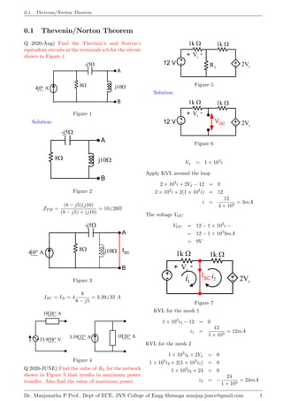
1. 0.1. Thevenin/Norton Theorem
0.1 Thevenin/Norton Theorem
Q 2020-Aug) Find the Thevinin’s and Norton’s
equivalent circuits at the terminals a-b for the circuit
shown in Figure 1.
j10
B
A
4 0 A
8
-j5
Figure 1
Solution:
j10
B
A
8
-j5
Figure 2
ZTH =
(8 − j5)(j10)
(8 − j5) + (j10)
= 10∠26Ω
j10
B
A
4 0 A
8
-j5
ISC
Figure 3
ISC = IN = 4
8
8 − j5
= 3.39∠32 A
10 26 A
33.9 58 V
3.39 32 A
10 26 A
Figure 4
Q 2020-JUNE) Find the value of RL for the network
shown in Figure 5 that results in maximum power
transfer. Also find the value of maximum power.
+
-
+
- 2Vx
Vx
-
+
1k 1k
RL
12 V
Figure 5
Solution:
VOC
12 V +
-
+
- 2Vx
Vx
-
+
1k 1k
Figure 6
Vx = 1 × 10³
i
Apply KVL around the loop
2 × 10³
i + 2Vx − 12 = 0
2 × 10³
i + 2(1 × 10³
i) = 12
i =
12
4 × 103
= 3mA
The voltage VOC
VOC = 12 − 1 × 10³
i −
= 12 − 1 × 10³
3mA
= 9V
+
-
+
- 2Vx
Vx
-
+
1k 1k
ISC
1
i 2
i
Figure 7
KVL for the mesh 1
1 × 10³
i1 − 12 = 0
i1 =
12
1 × 103
= 12mA
KVL for the mesh 2
1 × 10³
i2 + 2Vx = 0
1 × 10³
i2 + 2(1 × 10³
i1) = 0
1 × 10³
i2 + 24 = 0
i2 = −
24
1 × 103
= 24mA
Dr. Manjunatha P Prof., Dept of ECE, JNN College of Engg Shimoga manjup.jnnce@gmail.com 1
2. 0.1. Thevenin/Norton Theorem
The short circuit current is
ISC = i1 − i2 = 12mA − (−24mA)
= 36mA
The Thevenin’s resistance is
RTH =
VOC
ISC
=
9
36mA
= 250 Ω
Maximum power is transferred when RL = RTH.
The current in the circuit is
i =
9
250 + 250
= 0.018A
Maximum power is
P = i2
RL = (0.018)2
× 250 = 81mW
+
-
250
9 V
B
R 250
L
Figure 8
Q 2020-EE-JUNE) Determine the Thevenin’s
equivalent of the circuit shown in Figure ??
5
x
0.1V
B
A
x
V
3
+
-
4 V
Figure 9
Solution:
Vx − 4
5
− 0.1Vx = 0
0.2Vx − 0.1Vx = 0.8
Vx =
0.8
0.1
= 8V = VOC
By shorting the terminals
Vx = 0
5
x
0.1V
B
A
x
V
3
+
-
4 V ISC
Figure 10
V1 − 4
5
−
V1
3
= 0
0.2V1 − 0.8 − 0.33V1 = 0
−0.1333V1 = 0.8
V1 = −
0.8
0.1333
= 6V
ISC =
V1
3
=
6
3
= 2A
ZSC =
VOC
ISC
=
8
2
= 4Ω
Q 2019-DEC) Find the Thevenin and Norton
equivalent for the circuit shown in Figure ?? with
respect terminals a-b.
-+
+
-
1
i
1
2i
6Ω 10Ω
20 V
A
B
6Ω
Figure 11
Solution:
Determine the Thevenin voltage VTH. Apply KVL
for the circuit shown in Figure 12.
By KVL around the loop
6i − 2i + 6i − 20 = 0
10i = 20
i = 2A
Voltage across AB VOC = VTH is
VOC = 6i = 6 × 2 = 12V
-+
+
-
1
i
1
2i
6Ω 10Ω
20 V
A
B
i
6Ω VOC
Figure 12
When dependant voltage sources are present
then Thevenin Resistance RTH is calculated
Dr. Manjunatha P Prof., Dept of ECE, JNN College of Engg Shimoga manjup.jnnce@gmail.com 2
3. 0.1. Thevenin/Norton Theorem
by determining the short circuit current at
terminals AB:
-+
+
-
1
i
1
2i
6Ω 10Ω
20 V
A
B
6Ω ISC
y
x
Figure 13
x − y = i1
KVL for loop x
12x − 2i1 − 6y − 20 = 0
12x − 2(x − y) − 6y = 20
10x − 4y = 20
KVL for loop y
−6x + 16y = 0
6x − 16y = 0
Solving the following simultaneous equations
10x − 4y = 20
6x − 16y = 0
x = 2.353 y = 0.882
ISC = y = 0.882A
Thevenin’s resistance is
RTH =
VTH
ISC
=
12
0.882
= 13.6Ω
Thevenin and Norton equivalent circuits as shown
in Figure 14
+
-
13.6Ω
12 V
A
B
13.6Ω
0.882 A
A
B
Thevenin’s Equivalent Norton’s Equivalent
Figure 14
Q 2019-DEC) Determine the current through the
load resistance using Norton’s theorem for the
circuit shown in Figure 15.
L
I
3
4 V
A
B
1
2
8
L
R
1 A
+
-
10
Figure 15
Solution:
3 A
B
2
8
10
RTH
Figure 16
RTH = 11 Ω
L
I
3
4 V
A
B
2
8
1 A
+
-
10
V1
V2
Figure 17
V1 = 4
V2 − V1
3
+ 1 = 0
V2 − 4
3
+ 1 = 0
V2 − 4 + 3 = 0
V2 = 1
+
-
11
1 V
A
B
0.09 A
A
B
Thevenin’s Equivalent Norton’s Equivalent
11
Figure 18
Q 2019-Dec) Obtain the Thevenin’s equivalent
network for the circuit shown in Figure 19.
j24
j60
12
21 50
30
20 0 V
Dr. Manjunatha P Prof., Dept of ECE, JNN College of Engg Shimoga manjup.jnnce@gmail.com 3
4. 0.1. Thevenin/Norton Theorem
Figure 19
Solution:
B
RTH
A
j24 j60
12
21
50
30
Figure 20
RTH =
21(12 + j24)
21 + 12 + j24
+
50(30 + j60)
50 + 30 + j60
= (12.26 + j6.356) + (30 + j15))
= 42.26 + j21.356Ω
j24
j60
12
21 50
30
VAB
20 0 V
1
I 2
I
Figure 21
I1 =
20
33 + j24
= 0.49∠ − 36
I2 =
20
80 + j60
= 0.2∠ − 36.87
VAB = I1 × 21 − I2 × 50
= 0.49∠ − 36 × 21 − 0.2∠ − 36.87 × 50
= 0.49∠ − 36 × 21 − 0.2∠ − 36.87 × 50
= 0.328∠ − 8.457
42.26+j21.356
0.328 8.45 V
0.07 35 A
42.26+j21.356
Figure 22
Q 2019-JUNE) Obtain the Thevenin’s equivalent
across A and B for the circuit shown in Figure 23.
B
A
j8Ω
10
j10
-j8Ω
10 0 V
3 0 V
Figure 23
Solution:
RTH = j10 +
(10 + j8)(−j8)
(10 + j8 − j8)
= j10 + (6.4 − j8)
= 6 + j2Ω
B
RTH
A
j8Ω
10
j10
-j8Ω
Figure 24
V1 − 10
(10 + j8)
+
V1
(−j8)
+
V1 − 3
(j10)
= 0
V1[0.078∠ − 38.66 + 0.125∠90 + 0.1∠ − 90]
+0.78∠141 + 0.3∠90 = 0
0.0653∠ − 21.28V1 = −0.9964∠127.46
V1 =
−0.9964∠127.46
0.0653∠ − 21.28
V1 = 15.25∠ − 31.26
B
A
j8Ω
10
j10
-j8Ω
10 0 V
3 0 V
ISC
V1
Figure 25
ISC =
V1 − 3
(j10)
=
(15.25∠ − 31.26) − 3
j10
= 1.278∠ − 128.25
Dr. Manjunatha P Prof., Dept of ECE, JNN College of Engg Shimoga manjup.jnnce@gmail.com 4
5. 0.1. Thevenin/Norton Theorem
VOC = ISCZN
= 1.278∠ − 128.25(6 + j2)
= 8.08∠ − 109.815
+
-
8.08 109.81 V
6+j2
IN
B
A
1.278128.28 A
6+j2
Figure 26
Q 2019-JUNE) Find the value of ZL in the circuit
shown in Figure 27 using maximum power transfer
theorem and hence the maximum power.
j6Ω
B
A
5
-j8Ω
50 0 V
ZL
Figure 27
Solution:
B
RTH
A
j6Ω
5
-j8Ω
Figure 28
RTH =
(5 + j6)(−j8)
(5 + j6 − j8)
= 11 − j3.586Ω
B
A
5
-j8Ω
50 0 V
j6Ω
i
Figure 29
i =
50
(5 + j6 − j8)
= 9.28∠21.8
VOC = i(−j8)
= 9.28∠21.8(−j8)
= 74.24∠ − 68.2
+
-
74.24 68.2 V
11-j3.586
11+j3.586
Figure 30
Maximum Power is transferred when
RTH = RL
11 − j3.586Ω = 11 + j3.586Ω
Current through the load is
iL =
74.24∠ − 68.2
(11 − j3.586) + (11 + j3.586)
= 3.374A
Maximum Power transferred through the load is
PL = i2
LRL = (3.374)2
(11 + j3.586)
= 131.7∠18
Q 2019-JAN) Find the value of R for which the
power transferred across AB of the circuit shown
in Figure 31 is maximum and the maximum power
power transferred.
3
2
B
A R 4
20 V
1
10 V
+
-
+
-
Figure 31
Solution:
First remove the R from the network and determine
the VTH and RTH the details are as shown in Figure
32. The voltage across AB is the potential difference
between AB.
i1 =
10
3
The potential at A is
VA =
10
3
× 2Ω = 6.667V
Dr. Manjunatha P Prof., Dept of ECE, JNN College of Engg Shimoga manjup.jnnce@gmail.com 5
6. 0.1. Thevenin/Norton Theorem
i2 =
20
7
The potential at B is
VB =
20
7
× 3 = 8.571V
The potential at B is
VAB = VA − VB = 6.667V − 8.571V = −1.9V
3
2
B
A 4
20 V
1
10 V
+
-
+
-
Figure 32
To determine RTH the details are as shown in Figure
75. The 10Ω and 5Ω are in parallel which is in series
with 2Ω.
RTH = (1||2) + (3||4) = 0.667 + 1.714 = 2.381Ω
3
2
B
A 4
1
RAB
Figure 33
0.798 A
A
B
Norton’s
Equivalent
+
-
2.381
VTH
=1.9
A
B
Thevenin’s
Equivalent
2.381
Figure 34
IL =
1.9V
2.381 + 2.381
= 0.4A
PL = (0.4)2
× 2.381 = 0.381W
L
I
+
-
A
B
VTH =1.9
2.381
2.381
Figure 35
2018 Dec JUNE 2013-JUNE MARCH-2000 ) Find
the current through 6 Ω resistor using Norton’s
theorem for the circuit shown in Figure 36.
6Ω
B
A
4Ω
+
-
20 V
6Ix
5Ω
+-
Ix
Figure 36
Solution:
Determine the VOC at the terminal AB. When the
resistor is removed from the terminals AB then the
circuit is as shown in Figure 37. Apply KVL around
the loop
4Ix − 6Ix + 6Ix − 20 = 0
Ix =
20
4
= 5A
VOC = 5A × 6 = 30V
6Ω
B
A
4Ω
+
-
20 V
6Ix
+-
Ix
VOC
Figure 37
When the terminals AB short circuited then 6 Ω
resistor is also shorted and no current flows through
resistor hence Ix = 0 hence 6Ix = 0. The circuit is
as shown in Figure 38. The Norton current is
ISC = IN =
20
4
= 5 A
6Ω
B
A
4Ω
+
-
20 V
6Ix
+-
Ix
ISC
Figure 38
Dr. Manjunatha P Prof., Dept of ECE, JNN College of Engg Shimoga manjup.jnnce@gmail.com 6
7. 0.1. Thevenin/Norton Theorem
ZN =
VOC
ISC
=
30
5
= 6Ω
The Thevenin and Norton circuits are as shown in
Figure 39
5 A
A
B
Norton’s
Equivalent
6Ω
+
-
6Ω
VTH
=30 V
A
B
Thevenin’s
Equivalent
Figure 39
Current through 5 Ω resistor is
I5 = 5 A
6
6 + 5
' 2.72 A
5 A
A
B
Norton’s
Equivalent
6Ω 5Ω
Figure 40
2018 Dec 2011-JULY) Find the value of ZL for which
maximum power is transfer occurs in the circuit
shown in Figure 41.
ZL
A
20 0 V
°
3Ω
-j4Ω
+
-
10Ω
B
+ -
10 45 V
°
Figure 41
Solution:
Determine the VOC at the terminal AB. When the
resistor is removed from the terminals AB then the
circuit is as shown in Figure 42. Apply KVL around
the loop
I =
20∠00
10 + 3 − j4
=
20∠00
13.6∠ − 17.10
= 1.47∠17.10
A
VOC = [1.47∠17.10
× (3 − j4)] − 10∠450
= [1.47∠17.10
× 5∠ − 53.130
] − 10∠450
= [7.35∠ − 36.30
] − 10∠450
= [5.923 − j4.5] − 7.07 − j7.07
= −1.147 − j11.42
= 11.47V ∠95.730
20 0 V
3
-j4
+
-
10
+ -
10 45 V
A
B
VOC
+
+
+
_
_
_
i
V1
Figure 42
ZTH =
(3 − j4) × 10
3 − j4 + 10
= 2.973 − j2.162Ω
A
3Ω
-j4Ω
10Ω
B
RTH
Figure 43
+
-
2.973-j2.162 Ω
11.45 95.65 V
− ° ZL
A
B
Figure 44
ZTH =
(3 − j4) × 10
3 − j4 + 10
= 2.973 − j2.162Ω
The maximum power is delivered when the load
impedance is complex conjugatae of the network
impedance. Thus
ZL = Z∗
TH = 2.973 + j2.162Ω
Dr. Manjunatha P Prof., Dept of ECE, JNN College of Engg Shimoga manjup.jnnce@gmail.com 7
8. 0.1. Thevenin/Norton Theorem
The current flowing in the load impedance is
IL =
11.47V ∠95.730
ZTH + ZL
=
11.47V ∠95.730
2.973 − j2.162 + 2.973 + j2.162
=
11.47V ∠95.730
2.973 + 2.973
=
11.47V ∠95.730
5.946
= 1.929∠95.730
The power delivered in the load impedance is
PL = I2
L × RL = 1.9222
× 2.973 = 11.46W
2018 Jan) Find the Thevenin equivalent for the
circuit shown in Figure 45 with respect terminals
a-b
VA
2kΩ
A
B
3kΩ
-
4000
x
v
4 V +
- x
v
+
Figure 45
Solution:
Determine the Thevenin voltage VTH for circuit
shown in Figure 46. Apply KCL for the node V1
Vx = VA
VA − 4
2kΩ
−
Vx
4kΩ
= 0
0.5 × 10⁻³
VA − 0.25 × 10⁻³
VA = 2mA
VA = 8V
VOC = 8V
VA
2kΩ
A
B
3kΩ
-
4000
x
v
4 V +
- x
v
+
Figure 46
Determine the short circuit by shorting the output
terminals AB for circuit shown in Figure 47. Apply
KCL for the node V1. It is observed that Vx = 0 V ,
hence dependent current source becomes zero.
VA − 4
2kΩ
−
Vx
4kΩ
+
VA
3kΩ
= 0
0.5 × 10⁻³
VA + 0.333 × 10⁻³
VA = 2mA
0.833VA = 2
VA = 2.4V
ISC =
2.4V
3kΩ
= 0.8mA
VA
2kΩ
A
B
3kΩ
4000
x
v
4 V +
- ISC
Figure 47
ZTH =
VOC
ISC
=
8
0.8mA
= 10kΩ
Thevenin and Norton circuits are as shown in Figure
48
+
-
10kΩ
8 V
A
B
0.8 mA
A
B
Thevenin’s Equivalent Norton’s Equivalent
10kΩ
Figure 48
—————
Q 2017-Jan) What value of impedance ZL results
in maximum power transfer condition for the
network shown in Figure 49. Also determine the
corresponding power.
ZL
A
25 0 V
j6
+
-
2
B
25 50 V
+-
6
Figure 49
Solution:
Dr. Manjunatha P Prof., Dept of ECE, JNN College of Engg Shimoga manjup.jnnce@gmail.com 8
9. 0.1. Thevenin/Norton Theorem
ZTH =
VOC
ISC
= 2||(6 + j6)Ω
=
2(6 + j6)
(2 + 6 + j6)
= 1.68 + j0.24
A
j6
2
B
6 RTH
Figure 50
i =
25
8 + j6
= 2.5∠ − 36.87
V1 = i × (6 + j6) = 2.5∠ − 36.87 × (6 + j6)
= 21.21∠8.31V
VOC = VAB = V1 − 25∠50
= 21.21∠8.31 − 25∠50
= 16.82∠ − 73
A
25 0 V
j6
+
-
2
B
25 50 V
+-
6
V1
Figure 51
+
-
1.68-j0.24
16.82 73 V
Figure 52
+
- ZL
=
A
B
16.82 73 V
1.68+j0.24
1.68-j0.24
Figure 53
2017 Jan, 2014-JAN) Find the Thevenin’s equivalent
of the network as shown in Figure 54
5Ω
x
V
4
3Ω 10 A
B
A
x
V
+
−
3Ω V1
V2
Figure 54
Solution:
Using node analysis the following equations are
written
V1
6
+
V1 − V2
5
− 10 = 0
V1[0.166 + 0.2] − 0.2V2 = 10
0.366V1 − 0.2V2 = 10
V2 − V1
5
−
Vx
4
= 0
−0.2V1 + 0.2V2 − 0.25Vx = = 0
Vx =
V1
6
× 3 = 0.5V1
−0.2V1 + 0.2V2 − 0.25Vx = 0
−0.2V1 + 0.2V2 − 0.25 × 0.5V1 =
−0.325V1 + 0.2V2 = 0
0.366V1 − 0.2V2 = 10
−0.325V1 + 0.2V2 = 0
V1 = 243.93 V V2 = 396.3 V
VTH = V2 = 396.3 V
5Ω
x
V
4
3Ω 10 A
B
A
x
V
+
−
3Ω V1
V2
Figure 55
Dr. Manjunatha P Prof., Dept of ECE, JNN College of Engg Shimoga manjup.jnnce@gmail.com 9
10. 0.1. Thevenin/Norton Theorem
5Ω
x
V
4
3Ω 10 A
B
A
x
V
+
−
3Ω V1
V2
Figure 56
Vx =
10 × 5
11
× 3 = 13.636
ISC =
Vx
4
+ 10 ×
6
11
=
13.636
4
+ 5.45 = 3.41 + 5.45
= 8.86A
RTH =
VTH
ISC
=
396.3
13.636
= 44.01Ω
Q 2016-JUNE) Obtain the Thevenin’s equivalent
of the circuit shown in Figure 57 and thereby
find current through 5Ω resistor connected between
terminals A and B.
B
A
10
j10
-j5Ω
10 0 V
3 0 V
Figure 57
Solution:
RTH = j10 +
(10)(−j5)
(10 − j5)
= j10 + (2 − j4)
= 2 + j6Ω
B
RTH
A
10
j10
-j5Ω
Figure 58
V1 − 10
(10)
+
V1
(−j5)
+
V1 − 3
(j10)
= 0
V1[0.1 + 0.2∠90 + 0.1∠ − 90]
−1 + 0.3∠90 = 0
0.141∠ − 45V1 = 1.04∠163.3
V1 =
1.04∠163.3
0.141∠ − 45
V1 = 7.37∠ − 151.7
B
A
10
j10
-j5Ω
10 0 V
3 0 V
ISC
V1
Figure 59
ISC =
V1 − 3
(j10)
=
(7.37∠ − 151.7) − 3
j10
= 1.01∠110
VOC = ISCZN
= 1.01∠110(2 + j6)
= 6.38∠ − 17
+
- 6.38 17 V
2+j6
+
- 6.38 17 V
2+j6
5
Figure 60
I = j
6.38∠ − 17
(7 + j6)
= 0.69∠ − 57.6
Q 2015-Jan) For the network shown in Figure 61
draw the Thevenin’s equivalent circuit.
Dr. Manjunatha P Prof., Dept of ECE, JNN College of Engg Shimoga manjup.jnnce@gmail.com 10
11. 0.1. Thevenin/Norton Theorem
Ix
4
20 V
+ -
-+
6
6Ix
M
N
Figure 61
Solution:
Ix
4
20 V
+ -
-+
6
6Ix
M
N
Figure 62
−6Ix + 6Ix − 20 + 4Ix = 0
Ix =
20
4
= 5A
VOC = Ix × 6 = 5 × 6
= 30V
ISC = IN =
20
4
= 5 A
RTH =
VOC
ISC
=
30
5
= 6 Ω
ISC 4
20 V
+ -
M
N
ISC
Ix
4
20 V
+ -
-+
6
6Ix
M
N
Figure 63
+
-
6
30 V
B
Figure 64: Thevinin Circuit
Q 2014-JUNE) Find the value of load resistance
when maximum power is transferred across it and
also find the value of maximum power transferred
for the network of the circuit shown in Figure 65.
1.333
4
5 V
B
A
RL
+
- 2 A
+-
2 V
8
Figure 65
Solution:
1.333
4
B
A
8
Figure 66
ZTH = 1.333 +
8 × 4
8 + 4
= 1.333 + 2.6667 = 4Ω
V1 − 5
8
+
V1
4
+
V1 − 2
1.333
− 2 = 0
V1[0.125 + 0.25 + 0.75] − 0.625 − 1.5 − 2 = 0
V1[0.125 + 0.25 + 0.75] − 0.625 − 1.5 − 2 =
4.125
1.125
V1 = 3.666
ISC =
V1 − 2
1.333
=
3.6366 − 2
1.333
= 1.25
VOC = ISCZTH = 1.25 × 4 = 5
1.333
4
5 V
B
A
+
- 2 A
+-
2 V
8 V1
Figure 67
Pmax =
V 2
OC
RL
=
52
4
= 6.25W
Dr. Manjunatha P Prof., Dept of ECE, JNN College of Engg Shimoga manjup.jnnce@gmail.com 11
12. 0.1. Thevenin/Norton Theorem
+
-
4
VTH
=5
A
B
Thevenin’s
Equivalent
L
I
+
-
VTH
=5
A
B
4
4
Figure 68
Q 2014-JUNE) Find the current through 16 Ω
resistor using Nortons theorem for the circuit shown
in Figure 69.
6Ω
B
A
10Ω
+
-
40 V 0.8Ix
16Ω
I x
Figure 69
Solution:
Determine the VOC at the terminal AB. When the
resistor is removed from the terminals AB then
Ix = 0
VOC = 40 V
V1 6Ω
B
A
10Ω
+
-
40 V 0.8Ix
VOC
I x
Figure 70
Determine the VOC at the terminal AB by shorting
output terminals AB. Apply node analysis for the
circuit shown in Figure 71.
Ix =
V1
6
V1 − 40
10
+
V1
6
+ 0.8Ix = 0
V1
10
+
V1
6
+ 0.8
V1
6
= 0
0.4V1 = 4
V1 = 10
ISC = IN =
10
6
= 1.666 A
6Ω
B
A
10Ω
+
-
40 V 0.8Ix ISC
I x
Figure 71
ZN =
VOC
ISC
=
40
1.666
= 24Ω
1.667 A
A
B
Norton’s
Equivalent
24Ω
+
-
24Ω
VTH =40 V
A
B
Thevenin’s
Equivalent
Figure 72
Current through 16 Ω resistor is
I16 = 1.666 A
24
24 + 16
' 1 A
1.667 A
A
B
Norton’s
Equivalent
24Ω 16Ω
Figure 73
———————
Q 2014-JAN) State maximum power transfer
theorem. For the circuit shown in Figure 74 what
should be the value of R such that maximum power
transfer can take place from the rest of the network.
Obtain the amount of this power
5Ω
2Ω
5 A
B
A R 10Ω
24 V
Figure 74
Solution:
Dr. Manjunatha P Prof., Dept of ECE, JNN College of Engg Shimoga manjup.jnnce@gmail.com 12
13. 0.1. Thevenin/Norton Theorem
First remove the R from the network and determine
the VTH and RTH the details are as shown in Figure
75. The voltage across AB is the potential difference
between AB.
The potential at A is
VA = 5A × 2Ω = 10V
The potential at B is
VB =
24
15
× 5 = 8V
The potential at B is
VAB = VA − VB = 10V − 8V = 2V
5Ω
2Ω
5 A
B
A 10Ω
24 V
Figure 75
To determine RTH the details are as shown in Figure
75. The 10Ω and 5Ω are in parallel which is in series
with 2Ω.
RTH = 2 + (10||5) = 2 + 3.333 = 3.333Ω
5Ω
2Ω
B
A RAB
10Ω
Figure 76
0.375 A
A
B
Norton’s
Equivalent
5.33Ω
+
-
5.33Ω
VTH =2
A
B
Thevenin’s
Equivalent
Figure 77
L
I
+
-
5.33Ω
VTH =2
A
B
5.33Ω
Figure 78
—————————-
——————————–
Q 2012-JUNE) State Thevenin’s theorem. For the
circuit shown in Figure 79 find the current through
RL using Thevenin’s theorem.
1Ω
L
R 13
= Ω
10 A
B
A
2Ω V1
+
-
2Ω
10 V
Figure 79
Solution:
1Ω
10 A
B
A
2Ω V1
+
-
2Ω
10 V
Figure 80
By node analysis VTH is
V1 − 10
2
+
V1
2
− 10 = 0
V1 = 10 + 5 = 15V = ETH
RTH is
RTH = 1 +
2 × 2
2 + 2
= 2Ω
1Ω
2Ω V1
2Ω TH
R
A
B
Dr. Manjunatha P Prof., Dept of ECE, JNN College of Engg Shimoga manjup.jnnce@gmail.com 13
14. 0.1. Thevenin/Norton Theorem
Figure 81
L
R 13
= Ω
B
A
+
-
TH
R 2
= Ω
TH
E =15V
Figure 82
The current through IL is
IL =
ETH
RTH + RL
=
15
2 + 13
= 1A
—————————-
Q 2001-Aug, 2011-JAN) Obtain Thevenin and
Norton equivalent circuit at terminals AB for the
network shown in Figure 83 Find the current
through 10 Ω resistor across AB.
10Ω
B
A
5 30 A
°
5Ω
j5Ω
5Ω
j5Ω
Figure 83
Solution:
10Ω
B
A
5 30 A
°
5Ω
j5Ω
5Ω
j5Ω
Figure 84
IN
10Ω
B
A
5 30 A
°
5Ω
j5Ω
Figure 85
The Norton’s current IN is
IN = 5∠30 ×
5 + j5
10 + 5 + j5
= 5∠30 ×
7.07∠45
15.81∠18.43
= 2.236∠56.57◦
A
10Ω
B
A
5Ω
j5Ω
5Ω
j5Ω
RTH
Figure 86
ZN =
(5 + j5) × (15 + j5)
5 + j5 + 15 + j5
=
7.07∠45 × 15.81∠18.43
22.36∠26.56
= 5∠36.87◦
Ω
The Norton Equivalent circuit is as shown in Figure
87
IN
B
A
2.33 56.57 A
° 536.87° Ω
Figure 87
The Thevenin’s Equivalent
VTH = IN × ZN = 2.236∠56.57◦
A × 5∠36.87◦
Ω
= 11.18∠93.44◦
Ω
VTH = IN × ZN = 2.236∠56.57◦
Atimes5∠36.87◦
Ω
The Thevenin’s Equivalent circuit is as shown in
Figure 88
+
-
536.87° Ω
11.18 93.34 V
° 10 Ω
Figure 88
Current through load 10 is Ω
Dr. Manjunatha P Prof., Dept of ECE, JNN College of Engg Shimoga manjup.jnnce@gmail.com 14
15. 0.1. Thevenin/Norton Theorem
IL =
11.18∠93.43
5∠36.87 + 10
=
11.18∠93.43
4 + j3 + 10
=
11.18∠93.43
14.31∠12.1
◦
= 0.781∠81.34◦
—————————-
Q 2000-July) Obtain Thevenin and Norton equiva-
lent circuit at terminals AB for the network shown
in Figure 89. Find the current through 10 Ω resistor
across AB
-j10Ω
B
A
10 0 V
°
3Ω
j4Ω
+
-
10Ω
Figure 89
Solution:
B
10 0 V
°
3Ω
j4Ω
+
-
10Ω
A
-j10Ω
Figure 90
I(13 + j4) − 10 = 0
I(13.6∠17.1) = 10
I =
10
13.6∠17.1
I = 0.7352∠ − 17.1
VTH = I × (3 + j4) = (0.7352∠ − 17.1)(5∠53.13)
= 3.676∠36.03
B
RTH
10Ω
3Ω
j4Ω
A
-j10Ω
Figure 91
ZTH = −j10 +
10 × (3 + j4)
10 + 3 + j4
= −j10 +
30 + j40
13 + j4
= 10 +
50∠53.13
13.6∠17.027
= −j10 + 3.6762∠36.027◦
Ω
= −j10 + 2.9731 + j2.1622Ω
= 2.9731 − j7.8378Ω
= 8.3828∠ − 69.227Ω
+
-
8.3828 69.22
− Ω
3.67 36.027 V
°
Figure 92
Nortons equivalent circuit is ISC and ZTH which
are as shown in Figure 93
ISC =
VTH
ZTH
=
3.676∠36.03
8.3828∠ − 69.227
= 0.4385∠105.257
IN
B
A
2.33 56.57 A
° 8.3828 69.22
− Ω
Figure 93
—————————-
Q 2001-March) For the circuit shown in Figure
94 determine the load current IL using Norton’s
theorem .
-j2Ω
B
A
10 0 V
°
j3Ω
10Ω
5Ω
5 90 V
°
IL
Figure 94
Solution:
Determine the open circuit voltage VTH for the
circuit is as shown in Figure 101. Apply KVL
around the loop
Dr. Manjunatha P Prof., Dept of ECE, JNN College of Engg Shimoga manjup.jnnce@gmail.com 15
16. 0.1. Thevenin/Norton Theorem
x(j3 − j2) + 5∠90o
− 10∠0o
=
jx + j5 − 10 =
jx = 10 − j5
x = −j(10 − j5)
x = −5 − j10
x = 11.18∠ − 116.56o
The voltage VTH is the voltage between AB
VTH = 10∠0o
− j3x
= 10 − j3(−5 − j10)
= −20 + j15
= 25∠143.13o
-j2Ω
B
A
10 0 V
°
j3Ω
10Ω
5 90 V
°
x
Figure 95
The Thevenin impedance ZTH for the circuit is as
shown in Figure ?? is
ZTH =
j3 × (−j2)
j1
=
6
j1
= 6∠ − 90o
B
RTH
A
-j2Ω
j3Ω
Figure 96
The Thevenin circuit is as shown in Figure 97. The
current through the load is
IL =
25∠143.13o
5 − j6
=
25∠143.13o
7.8∠ − 50.2o
= 3.2∠193.3o
PL = I2
LRL
PL = (3.2)2
× 5
= 51.2W
+
- 25143.13 V
°
-j6 Ω
5Ω
L
I
Figure 97
IN
B
A
4.167 233.13 A
° 6
j
− Ω
Figure 98
—————————-
Q 2000-March) What should be the value of pure
resistance to be connected across the terminals A
and B in the network shown in Figure 99 so that
maximum power is transferred to the load? What is
the maximum power?
j10Ω
B
A
100 0 V
°
j10Ω
-j20Ω
Figure 99
Solution:
The open circuit voltage VTH for the circuit is as
shown in Figure 101 is
x(j10 − j20) − 100∠0o
=
x =
100∠0o
−j10
x = j10
VTH = j10 × −j20
= 200V
Dr. Manjunatha P Prof., Dept of ECE, JNN College of Engg Shimoga manjup.jnnce@gmail.com 16
17. 0.1. Thevenin/Norton Theorem
j10Ω
B
A
100 0 V
°
j10Ω
-j20Ω
x
Figure 100
The Thevenin impedance ZTH for the circuit is as
shown in Figure ?? is
ZTH = j10 +
j10 × (−j20)
j10 − j10
= j10 +
200
−j10
= j10 +
100∠0o
−j10
= j10 + j20
= j30
j10Ω
B
A
100 0 V
°
j10Ω
-j20Ω
x
Figure 101
The Thevenin circuit is as shown in Figure 102. The
current through the load is
IL =
200
30 + j30
=
200
42.43∠45o
= 4.714∠ − 45o
PL = I2
LRL
= (4.714)2
× 30
= 666.6W
+
-
200 0 V
°
j30 Ω
30 Ω
L
I
Figure 102
—————————-
Q 2000-FEB) What should be the value of pure
resistance to be connected across the terminals A
and B in the network shown in Figure 103 so that
maximum power is transferred to the load? What is
the maximum power?
B
A
10 0 V
° 5 90 V
°
10 30
− ° Ω
5 60° Ω
Figure 103
Solution:
The open circuit voltage VTH for the circuit is as
shown in Figure 101 is
x(5∠60o
+ 10∠ − 30o
) + 5∠90o
− 10∠0o
= 0
x(2.5 + j4.33 + 8.66 − j5) + j5 − 10 = 0
x(11.16 − j0.67) = 10 − j5
=
10 − j5
11.16 − j0.67
=
11.18∠ − 26.56
11.18∠ − 34.36
= 1∠ − 23.13
VAB = 10∠0o
− x(5∠60o
)
= 10 − (1∠ − 23.13)(5∠60o
)
= 10 − (5∠36.87)
= 10 − (4 + j3)
= 6 − j3
VTH = 6.7∠ − 26.56)
B
A
10 0 V
° 5 90 V
°
10 30
− ° Ω
5 60° Ω
x
Figure 104
The Thevenin impedance ZTH for the circuit is as
shown in Figure 105 is
Dr. Manjunatha P Prof., Dept of ECE, JNN College of Engg Shimoga manjup.jnnce@gmail.com 17
18. 0.1. Thevenin/Norton Theorem
ZTH =
5∠60o × 10∠ − 30o
5∠60o + 10∠ − 30o
ZTH = j10 +
j10 × (−j20)
j10 − j10
=
50∠30o
(2.5 + j4.33) + (8.66 − j53)
=
50∠30o
11.18∠ − 34.36o
= 4.47∠26.56o
= 4 + j2
B
RTH
A
5 60° Ω
10 30
− ° Ω
Figure 105
The load impedance is 4-j2 Ω
The Thevenin circuit is as shown in Figure 106. The
current through the load is
IL =
6.708∠ − 26.56
4 + j2 + 4 − j2
=
6.708∠ − 26.56
8
= 0.8385∠ − 26.65o
PL = I2
LRL
= (0.8385)2
× 4
= 2.8123W
0
6.708 26.56
∠ −
4+j2Ω
4-j2Ω
Figure 106
Important: All the diagrams are redrawn and solutions are prepared. While
preparing this study material most of the concepts are taken from some text books
or it may be Internet. This material is just for class room teaching to make
better understanding of the concepts on Network analysis: Not for any commercial
purpose
Dr. Manjunatha P Prof., Dept of ECE, JNN College of Engg Shimoga manjup.jnnce@gmail.com 18