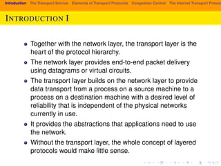
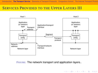
The document provides an overview of the transport layer in computer networks. It discusses the key services provided by the transport layer, including reliable data transmission and isolating applications from the underlying network technology. It introduces some common transport layer protocols like TCP and UDP, and describes important transport layer concepts such as connection-oriented vs. connectionless services, transport service primitives, and elements that transport protocols must address like error control and flow control.
RANDOM ACCESS PROTOCOL IN COMMUNICATION AMOGHA A K
In random access ,each station has right to send the data. However , if more than one station tries to send ,collision will occur .To avoid this collision , protocols came into existence.
In random access method , no stations are superior & none is assigned the control over the other .
When a station has a data to send , it uses a procedure defined by a protocol whether to send or not .
The data link layer, or layer 2, is the second layer of the seven-layer OSI model of computer networking. This layer is the protocol layer that transfers data between adjacent network nodes in a wide area network (WAN) or between nodes on the same local area network (LAN) segment.
explanation of :-difference between udp and tcp,different network models,modes of communication,different layers with help of examples.network layers and how it works
A Machine Learning based Network Sharing System Design with MPTCPIJMREMJournal
The information and communication technologies (ICT) integrate different types of wireless communication to
provide IT-enabled services and applications. The great majority end devices are equipped with multiple network
interfaces such as Wi-Fi and 4G. Our goal is to integrate the available network interfaces and technologies to
enhance seamless communication efficiency and increase resources utilization. We proposed a heterogeneous
network management algorithm based on machine learning methods which includes roaming and sharing
functions. The roaming function provides the multiple network resources in physical and media access control
layers. The sharing function supports multiple network resources allocation and the service handover process
based on the Multi-Path TCP protocol. The simulation result also shows that the proposed scheme can increase
the network bandwidth utilization effectively. The sharing system could be used in home, mobile and vehicular
environments to realize ubiquitous social sharing networks.
A Machine Learning based Network Sharing System Design with MPTCPIJMREMJournal
The information and communication technologies (ICT) integrate different types of wireless communication to provide IT-enabled services and applications. The great majority end devices are equipped with multiple network interfaces such as Wi-Fi and 4G. Our goal is to integrate the available network interfaces and technologies to enhance seamless communication efficiency and increase resources utilization. We proposed a heterogeneous network management algorithm based on machine learning methods which includes roaming and sharing functions. The roaming function provides the multiple network resources in physical and media access control layers. The sharing function supports multiple network resources allocation and the service handover process based on the Multi-Path TCP protocol. The simulation result also shows that the proposed scheme can increase the network bandwidth utilization effectively. The sharing system could be used in home, mobile and vehicular environments to realize ubiquitous social sharing networks.
Talhunt is a leader in assisting and executing IEEE Engineering projects to Engineering students - run by young and dynamic IT entrepreneurs. Our primary motto is to help Engineering graduates in IT and Computer science department to implement their final year project with first-class technical and academic assistance.
Project assistance is provided by 15+ years experienced IT Professionals. Over 100+ IEEE 2015 and 200+ yester year IEEE project titles are available with us. Projects are based on Software Development Life-Cycle (SDLC) model.
A Case Study on Ip Based Cdma Ran by Controlling RouterIJERA Editor
As communication plays an important role in day to day life, the effective and efficient data transmission is to be maintained. This paper mainly deals with implements a congestion control mechanism using Router control method for IP-RAN on CDMA cellular network. The Router control mechanism uses the features of CDMA networks using active Queue Management technique to reduce delay and to minimize the correlated losses. When utilizing these new personal tools and services to enrich our lives, while being mobile, we are using Mobile Multimedia applications. As new handsets, new technologies and new business models are introduced on the marketplace, new attractive multimedia services can and will be launched, fulfilling the demands. Because the number of multimedia services and even more so, the context in which the services are used is numerous, the following model is introduced in order to simplify and clarify how different services will evolve, enrich our lives and fulfill our desires.The proposed paper work is to be realized using Matlab platform.
This is inspired from Tom Mitchell's book on Machine Learning. You can achieve a bit exact implementation of the back propagation algorithm if you follow the code in this.
A simple client-server application in java in which a client sends a message to a server and the server tries to be funny by sending back a funny response.
Democratizing Fuzzing at Scale by Abhishek Aryaabh.arya
Presented at NUS: Fuzzing and Software Security Summer School 2024
This keynote talks about the democratization of fuzzing at scale, highlighting the collaboration between open source communities, academia, and industry to advance the field of fuzzing. It delves into the history of fuzzing, the development of scalable fuzzing platforms, and the empowerment of community-driven research. The talk will further discuss recent advancements leveraging AI/ML and offer insights into the future evolution of the fuzzing landscape.
Saudi Arabia stands as a titan in the global energy landscape, renowned for its abundant oil and gas resources. It's the largest exporter of petroleum and holds some of the world's most significant reserves. Let's delve into the top 10 oil and gas projects shaping Saudi Arabia's energy future in 2024.
Cosmetic shop management system project report.pdfKamal Acharya
Buying new cosmetic products is difficult. It can even be scary for those who have sensitive skin and are prone to skin trouble. The information needed to alleviate this problem is on the back of each product, but it's thought to interpret those ingredient lists unless you have a background in chemistry.
Instead of buying and hoping for the best, we can use data science to help us predict which products may be good fits for us. It includes various function programs to do the above mentioned tasks.
Data file handling has been effectively used in the program.
The automated cosmetic shop management system should deal with the automation of general workflow and administration process of the shop. The main processes of the system focus on customer's request where the system is able to search the most appropriate products and deliver it to the customers. It should help the employees to quickly identify the list of cosmetic product that have reached the minimum quantity and also keep a track of expired date for each cosmetic product. It should help the employees to find the rack number in which the product is placed.It is also Faster and more efficient way.
Student information management system project report ii.pdfKamal Acharya
Our project explains about the student management. This project mainly explains the various actions related to student details. This project shows some ease in adding, editing and deleting the student details. It also provides a less time consuming process for viewing, adding, editing and deleting the marks of the students.
Forklift Classes Overview by Intella PartsIntella Parts
Discover the different forklift classes and their specific applications. Learn how to choose the right forklift for your needs to ensure safety, efficiency, and compliance in your operations.
For more technical information, visit our website https://intellaparts.com
Final project report on grocery store management system..pdfKamal Acharya
In today’s fast-changing business environment, it’s extremely important to be able to respond to client needs in the most effective and timely manner. If your customers wish to see your business online and have instant access to your products or services.
Online Grocery Store is an e-commerce website, which retails various grocery products. This project allows viewing various products available enables registered users to purchase desired products instantly using Paytm, UPI payment processor (Instant Pay) and also can place order by using Cash on Delivery (Pay Later) option. This project provides an easy access to Administrators and Managers to view orders placed using Pay Later and Instant Pay options.
In order to develop an e-commerce website, a number of Technologies must be studied and understood. These include multi-tiered architecture, server and client-side scripting techniques, implementation technologies, programming language (such as PHP, HTML, CSS, JavaScript) and MySQL relational databases. This is a project with the objective to develop a basic website where a consumer is provided with a shopping cart website and also to know about the technologies used to develop such a website.
This document will discuss each of the underlying technologies to create and implement an e- commerce website.
Quality defects in TMT Bars, Possible causes and Potential Solutions.PrashantGoswami42
Maintaining high-quality standards in the production of TMT bars is crucial for ensuring structural integrity in construction. Addressing common defects through careful monitoring, standardized processes, and advanced technology can significantly improve the quality of TMT bars. Continuous training and adherence to quality control measures will also play a pivotal role in minimizing these defects.
Sachpazis:Terzaghi Bearing Capacity Estimation in simple terms with Calculati...Dr.Costas Sachpazis
Terzaghi's soil bearing capacity theory, developed by Karl Terzaghi, is a fundamental principle in geotechnical engineering used to determine the bearing capacity of shallow foundations. This theory provides a method to calculate the ultimate bearing capacity of soil, which is the maximum load per unit area that the soil can support without undergoing shear failure. The Calculation HTML Code included.
Explore the innovative world of trenchless pipe repair with our comprehensive guide, "The Benefits and Techniques of Trenchless Pipe Repair." This document delves into the modern methods of repairing underground pipes without the need for extensive excavation, highlighting the numerous advantages and the latest techniques used in the industry.
Learn about the cost savings, reduced environmental impact, and minimal disruption associated with trenchless technology. Discover detailed explanations of popular techniques such as pipe bursting, cured-in-place pipe (CIPP) lining, and directional drilling. Understand how these methods can be applied to various types of infrastructure, from residential plumbing to large-scale municipal systems.
Ideal for homeowners, contractors, engineers, and anyone interested in modern plumbing solutions, this guide provides valuable insights into why trenchless pipe repair is becoming the preferred choice for pipe rehabilitation. Stay informed about the latest advancements and best practices in the field.
1. Introduction The Transport Service Elements of Transport Protocols Congestion Control The Internet Transport Protocols: THE TRANSPORT LAYER
Muhammad Adil Raja
Roaming Researchers, Inc.
September 4, 2014
2. Introduction The Transport Service Elements of Transport Protocols Congestion Control The Internet Transport Protocols: OUTLINE
3. Introduction The Transport Service Elements of Transport Protocols Congestion Control The Internet Transport Protocols: INTRODUCTION I
Together with the network layer, the transport layer is the
heart of the protocol hierarchy.
The network layer provides end-to-end packet delivery
using datagrams or virtual circuits.
The transport layer builds on the network layer to provide
data transport from a process on a source machine to a
process on a destination machine with a desired level of
reliability that is independent of the physical networks
currently in use.
It provides the abstractions that applications need to use
the network.
Without the transport layer, the whole concept of layered
protocols would make little sense.
4. Introduction The Transport Service Elements of Transport Protocols Congestion Control The Internet Transport Protocols: INTRODUCTION II
In this lesson, we will study the transport layer in detail,
including its services and choice of API design to tackle
issues of reliability, connections and congestion control,
protocols such as TCP and UDP, and performance.
5. Introduction The Transport Service Elements of Transport Protocols Congestion Control The Internet Transport Protocols: THE TRANSPORT SERVICE I
We look at what kind of service is provided to the
application layer.
To make the issue of transport service more concrete, we
will examine two sets of transport layer primitives.
First comes a simple (but hypothetical) one to show the
basic ideas.
Then comes the interface commonly used in the Internet.
6. Introduction The Transport Service Elements of Transport Protocols Congestion Control The Internet Transport Protocols: SERVICES PROVIDED TO THE UPPER LAYERS I
The ultimate goal of the transport layer is to provide
efficient, reliable, and cost-effective data transmission
service to its users.
These services are used normally by the processes in the
application layer.
To achieve this, the transport layer makes use of the
services provided by the network layer.
The software and/or hardware within the transport layer
that does the work is called the transport entity.
The transport entity can be located in the operating system
kernel, in a library package bound into network
applications, in a separate user process, or even on the
network interface card.
The first two options are most common on the Internet.
7. Introduction The Transport Service Elements of Transport Protocols Congestion Control The Internet Transport Protocols: SERVICES PROVIDED TO THE UPPER LAYERS II
The (logical) relationship of the network, transport, and
application layers is illustrated in
Figure. ˙reffig:network-transport-app-layers.
8. layer that does the work is called the transport entity. The transport entity can
be located in the operating system kernel, in a library package bound into network
applications, in a separate user process, or even on the network interface card.
The first two options are most common on the Internet. The (logical) relationship
of the network, transport, and application layers is illustrated in Fig. 6-1.
Introduction The Transport Service Elements of Transport Protocols Congestion Control The Internet Transport Protocols: SERVICES PROVIDED TO THE UPPER LAYERS III
Host 1 Host 2
Application/transport
interface
Transport/network
interface
Application
(or session)
layer
Transport
entity
Transport
address
Network
address
Network layer
Application
(or session)
layer
Transport
entity
Network layer
Segment
Transport
protocol
Figure 6-1. The network, transport, and application layers.
FIGURE: The network transport and application layers..
Just as there are two types of network service, connection-oriented and con-nectionless,
there are also two types of transport service. The connection-oriented
transport service is similar to the connection-oriented network service in many
9. Introduction The Transport Service Elements of Transport Protocols Congestion Control The Internet Transport Protocols: SERVICES PROVIDED TO THE UPPER LAYERS IV
Just as there are two types of network service,
connection-oriented and con- nectionless, there are also
two types of transport service.
The connection-oriented transport service is similar to the
connection-oriented network service in many ways.
In both cases, connections have three phases:
establishment, data transfer, and release.
Addressing and flow control are also similar in both layers.
Furthermore, the connectionless transport service is also
very similar to the connectionless network service.
However, note that it can be difficult to provide a
connectionless transport service on top of a
connection-oriented network service, since it is inefficient
to set up a connection to send a single packet and then
tear it down immediately afterwards.
10. Introduction The Transport Service Elements of Transport Protocols Congestion Control The Internet Transport Protocols: SERVICES PROVIDED TO THE UPPER LAYERS V
if the transport layer service is so similar to the network
layer service, why are there two distinct layers?
Why is one layer not adequate?
The transport code runs entirely on the users’ machines,
but the network layer mostly runs on the routers, which are
operated by the carrier (at least for a wide area network).
What happens if the network layer offers inadequate
service?
What if it frequently loses packets?
What happens if routers crash from time to time?
The users have no real control over the network layer, so
they cannot solve the problem of poor service by using
better routers or putting more error handling in the data link
layer because they don’t own the routers.
11. Introduction The Transport Service Elements of Transport Protocols Congestion Control The Internet Transport Protocols: SERVICES PROVIDED TO THE UPPER LAYERS VI
The only possibility is to put on top of the network layer
another layer that improves the quality of the service.
If, in a connectionless network, packets are lost or
mangled, the transport entity can detect the problem and
compensate for it by using retransmissions.
If, in a connection-oriented network, a transport entity is
informed halfway through a long transmission that its
network connection has been abruptly terminated, with no
indication of what has happened to the data currently in
transit, it can set up a new network connection to the
remote transport entity.
Using this new network connection, it can send a query to
its peer asking which data arrived and which did not, and
knowing where it was, pick up from where it left off.
12. Introduction The Transport Service Elements of Transport Protocols Congestion Control The Internet Transport Protocols: SERVICES PROVIDED TO THE UPPER LAYERS VII
In essence, the existence of the transport layer makes it
possible for the transport service to be more reliable than
the underlying network.
Furthermore, the transport primitives can be implemented
as calls to library procedures to make them independent of
the network primitives.
The network service calls may vary considerably from one
network to another (e.g., calls based on a connectionless
Ethernet may be quite different from calls on a
connection-oriented WiMAX network).
Hiding the network service behind a set of transport
service primitives ensures that changing the network
merely requires replacing one set of library procedures
with another one that does the same thing with a different
underlying service.
13. Introduction The Transport Service Elements of Transport Protocols Congestion Control The Internet Transport Protocols: SERVICES PROVIDED TO THE UPPER LAYERS VIII
By virtue of the transportlayer, application programmers
can write code accord- ing to a standard set of primitives
and have these programs work on a wide variety of
networks.
This can be done without having to worry about dealing
with different network interfaces and levels of reliability.
If all real networks were flawless and all had the same
service primitives and were guaranteed never, ever to
change, the transport layer might not be needed.
However, in the real world it fulfills the key function of
isolating the upper layers from the technology, design, and
imperfections of the network.
For this reason, many people have made a qualitative
distinction between layers 1 through 4 on the one hand
and layer(s) above 4 on the other.
14. Introduction The Transport Service Elements of Transport Protocols Congestion Control The Internet Transport Protocols: SERVICES PROVIDED TO THE UPPER LAYERS IX
The bottom four layers can be seen as the transport
service provider, whereas the upper layer(s) are the
transport service user.
This distinction of provider versus user has a considerable
impact on the design of the layers and puts the transport
layer in a key position, since it forms the major boundary
between the provider and user of the reliable data
transmission service.
It is the level that applications see.
15. Introduction The Transport Service Elements of Transport Protocols Congestion Control The Internet Transport Protocols: TRANSPORT SERVICE PRIMITIVES I
To allow users to access the transport service, the
transport layer must provide some operations to
application programs, that is, a transport service interface.
Each transport service has its own interface.
In this section, we will first examine a simple (hypothetical)
transport service and its interface to see the bare
essentials.
In the following section, we will look at a real example.
The transport service is similar to the network service, but
there are also some important differences.
The main difference is that the network service is intended
to model the service offered by real networks, warts and
all.
16. Introduction The Transport Service Elements of Transport Protocols Congestion Control The Internet Transport Protocols: TRANSPORT SERVICE PRIMITIVES II
Real networks can lose packets, so the network service is
generally unreliable.
The connection-oriented transport service, in contrast, is
reliable.
Of course, real networks are not error-free, but that is
precisely the purpose of the transport layerÑto provide a
reliable service on top of an unreliable network.
As an example, consider two processes on a single
machine connected by a pipe in UNIX (or any other
interprocess communication facility).
They assume the connection between them is 100%
perfect.
They do not want to know about acknowledgements, lost
packets, congestion, or anything at all like that.
17. Introduction The Transport Service Elements of Transport Protocols Congestion Control The Internet Transport Protocols: TRANSPORT SERVICE PRIMITIVES III
What they want is a 100% reliable connection.
Process A puts data into one end of the pipe, and process
B takes it out of the other.
This is what the connection-oriented transport service is all
about – hiding the imperfections of the network service so
that user processes can just assume the existence of an
error-free bit stream even when they are on different
machines.
As an aside, the transport layer can also provide unreliable
(datagram) service.
However, there is relatively little to say about that besides
Ô“it’s datagrams”,
So we will mainly concentrate on the connection-oriented
transport service here.
18. Introduction The Transport Service Elements of Transport Protocols Congestion Control The Internet Transport Protocols: TRANSPORT SERVICE PRIMITIVES IV
Nevertheless, there are some applications, such as
client-server computing and streaming multimedia, that
build on a connectionless transport service, and we will say
a little bit about that later on.
A second difference between the network service and
transport service is whom the services are intended for.
The network service is used only by the transport entities.
Few users write their own transport entities, and thus few
users or programs ever see the bare network service.
In contrast, many programs (and thus programmers) see
the transport primitives.
Consequently, the transport service must be convenient
and easy to use.
consider the five primitives listed in Figure. ??.
19. Introduction The Transport Service Elements of Transport Protocols Congestion Control The Internet Transport Protocols: TRANSPORT SERVICE PRIMITIVES V
SEC. 6.1 THE TRANSPORT SERVICE 499
Primitive Packet sent Meaning
LISTEN (none) Block until some process tries to connect
CONNECT CONNECTION REQ. Actively attempt to establish a connection
SEND DATA Send information
RECEIVE (none) Block until a DATA packet arrives
DISCONNECT DISCONNECTION REQ. Request a release of the connection
Figure 6-2. The primitives for a simple transport service.
FIGURE: The primitives for a simple transport service.
blocks the server until a client turns up. When a client wants to talk to the server,
it executes a CONNECT primitive. The transport entity carries out this primitive by
blocking the caller and sending a packet to the server. Encapsulated in the pay-load
of this packet is a transport layer message for the server’s transport entity.
A quick note on terminology is now in order. For lack of a better term, we
will use the term segment for messages sent from transport entity to transport en-tity.
TCP, UDP and other Internet protocols use this term. Some older protocols
used the ungainly name TPDU (Transport Protocol Data Unit). That term is
20. Thus, segments (exchanged by the transport layer) are contained in packets
(exchanged by the network layer). In turn, these packets are contained in frames
(exchanged by the data link layer). When a frame arrives, the data link layer
processes the frame header and, if the destination address matches for local deliv-ery,
Introduction The Transport Service Elements of Transport Protocols Congestion Control The Internet Transport Protocols: TRANSPORT SERVICE PRIMITIVES VI
passes the contents of the frame payload field up to the network entity. The
network entity similarly processes the packet header and then passes the contents
of the packet payload up to the transport entity. This nesting is illustrated in
Fig. 6-3.
Frame
header
Packet
header
Segment
header
Segment payload
Packet payload
Frame payload
Figure 6-3. Nesting of segments, packets, and frames.
FIGURE: Nesting of segments, packets, and frames.
Getting back to our client-server example, the client’s CONNECT call causes a
CONNECTION REQUEST segment to be sent to the server. When it arrives, the
21. Introduction The Transport Service Elements of Transport Protocols Congestion Control The Internet Transport Protocols: BERKELEY SOCKETS I
SEC. 6.1 THE TRANSPORT SERVICE 501
Connect primitive
executed
ACTIVE
ESTABLISHMENT
PENDING
PASSIVE
ESTABLISHMENT
PENDING
PASSIVE
DISCONNECT
PENDING
ACTIVE
DISCONNECT
PENDING
IDLE
ESTABLISHED
IDLE
Disconnection
request segment
received
Disconnect
primitive
executed
Disconnect
primitive executed
Disconnection request
segment received
Connection request
segment received
Connection accepted
segment received
Connect primitive
executed
Figure 6-4. A state diagram for a simple connection management scheme.
Transitions labeled in italics are caused by packet arrivals. The solid lines show
the client’s state sequence. The dashed lines show the server’s state sequence.
systems, especially UNIX-based systems, and there is a socket-style API for Win-dows
called ‘‘winsock.’’
The primitives are listed in Fig. 6-5. Roughly speaking, they follow the mo-del
of our first example but offer more features and flexibility. We will not look
at the corresponding segments here. That discussion will come later.
Primitive Meaning
SOCKET Create a new communication endpoint
FIGURE: A state diagram for a simple connection management
scheme. Transitions labeled in italics are caused by packet arrivals.
The solid lines show the clients state sequence. The dashed lines
show the servers state sequence.
22. systems, especially UNIX-based systems, and there is a socket-style API for Win-dows
Introduction The Transport Service Elements of Transport Protocols Congestion Control The Internet Transport Protocols: BERKELEY SOCKETS II
called ‘‘winsock.’’
The primitives are listed in Fig. 6-5. Roughly speaking, they follow the mo-del
of our first example but offer more features and flexibility. We will not look
at the corresponding segments here. That discussion will come later.
Primitive Meaning
SOCKET Create a new communication endpoint
BIND Associate a local address with a socket
LISTEN Announce willingness to accept connections; give queue size
ACCEPT Passively establish an incoming connection
CONNECT Actively attempt to establish a connection
SEND Send some data over the connection
RECEIVE Receive some data from the connection
CLOSE Release the connection
Figure 6-5. The socket primitives for TCP.
FIGURE: The socket primitives for TCP.
23. Introduction The Transport Service Elements of Transport Protocols Congestion Control The Internet Transport Protocols: ELEMENTS OF TRANSPORT PROTOCOLS I
The transport service is implemented by a transport
protocol used between the two transport entities.
In some ways, transport protocols resemble the data link
protocols.
Both have to deal with error control, sequencing, and flow
control, among other issues.
However, significant differences between the two also exist.
These differences are due to major dissimilarities between
the environments in which the two protocols operate, as
shown in Figure. ??.
At the data link layer, two routers communicate directly via
a physical channel, whether wired or wireless, whereas at
the transport layer, this physical channel is replaced by the
entire network.
24. Introduction The Transport Service Elements of Transport Protocols Congestion Control The Internet Transport Protocols: ELEMENTS OF TRANSPORT PROTOCOLS II
This difference has many important implications for the
protocols:
1 Over point-to-point links such as wires or optical fiber, it is
usually not necessary for a router to specify which router it
wants to talk to – each outgoing line leads directly to a
particular router.
In the transport layer, explicit addressing of destinations is
required.
2 The process of establishing a connection over the wire of
Figure. ?? (a) is simple: the other end is always there
(unless it has crashed, in which case it is not there).
Either way, there is not much to do.
Even on wireless links, the process is not much different.
Just sending a message is sufficient to have it reach all other
destinations.
If the message is not acknowledged due to an error, it can
be resent.
25. Introduction The Transport Service Elements of Transport Protocols Congestion Control The Internet Transport Protocols: ELEMENTS OF TRANSPORT PROTOCOLS III
In the transport layer, initial connection establishment is
complicated.
3 When a router sends a packet over a link, it may arrive or
be lost, but it cannot bounce around for a while, go into
hiding in a far corner of the world, and suddenly emerge
after other packets that were sent much later.
If the network uses datagrams, which are independently
routed inside, there is a nonnegligible probability that a
packet may take the scenic route and arrive late and out of
the expected order, or even that duplicates of the packet will
arrive.
The consequences of the network’s ability to delay and
duplicate packets can sometimes be disastrous and can
require the use of special protocols to correctly transport
information.
26. Introduction The Transport Service Elements of Transport Protocols Congestion Control The Internet Transport Protocols: ELEMENTS OF TRANSPORT PROTOCOLS IV
4 The presence in the transport layer of a large and varying
number of connections with bandwidth that fluctuates as
the connections compete with each other may require a
different approach than we used in the data link layer.
508 THE TRANSPORT LAYER CHAP. 6
communicate directly via a physical channel, whether wired or wireless, whereas
at the transport layer, this physical channel is replaced by the entire network. This
difference has many important implications for the protocols.
Router Router
Network
Physical
communication channel Host
(a) (b)
Figure 6-7. (a) Environment of the data link layer. (b) Environment of the
transport layer.
FIGURE: (a) Environment of the data link layer. (b) Environment of the
transport layer.
For one thing, over point-to-point links such as wires or optical fiber, it is
usually not necessary for a router to specify which router it wants to talk to—each
outgoing line leads directly to a particular router. In the transport layer, explicit
27. Introduction The Transport Service Elements of Transport Protocols Congestion Control The Internet Transport Protocols: ADDRESSING I
Use of ports.
TSAP (Transport Service Access Point).
28. (Network Service Access Points). IP addresses are examples of NSAPs.
Introduction The Transport Service Elements of Transport Protocols Congestion Control The Internet Transport Protocols: Figure 6-8 illustrates the relationship between the NSAPs, the TSAPs, and a
ADDRESSING II
transport connection. Application processes, both clients and servers, can attach
themselves to a local TSAP to establish a connection to a remote TSAP. These
connections run through NSAPs on each host, as shown. The purpose of having
TSAPs is that in some networks, each computer has a single NSAP, so some way
is needed to distinguish multiple transport endpoints that share that NSAP.
Host 1 Host 2
Application
process
Application
layer
Transport
connection
TSAP 1522
TSAP 1208
NSAP
NSAP
Transport
layer
Network
layer
Data link
layer
Physical
layer
Server 1
Server 2
TSAP1836
Figure 6-8. TSAPs, NSAPs, and transport connections.
FIGURE: TSAPs, NSAPs, and transport connections.
29. Introduction The Transport Service Elements of Transport Protocols Congestion Control The Internet Transport Protocols: ADDRESSING III
A possible scenario for a transport connection is as follows:
1 A mail server process attaches itself to TSAP 1522 on host
2 to wait for an incoming call. How a process attaches
itself to a TSAP is out- side the networking model and
depends entirely on the local operating system. A call such
as our LISTEN might be used, for example.
2 An application process on host 1 wants to send an email
message, so it attaches itself to TSAP 1208 and issues a
CONNECT request. The request specifies TSAP 1208 on
host 1 as the source and TSAP 1522 on host 2 as the
destination. This action ultimately results in a transport
connection being established between the application
process and the server.
3 The application process sends over the mail message.
30. Introduction The Transport Service Elements of Transport Protocols Congestion Control The Internet Transport Protocols: ADDRESSING IV
4 The mail server responds to say that it will deliver the
message.
5 The transport connection is released.
31. Introduction The Transport Service Elements of Transport Protocols Congestion Control The Internet Transport Protocols: ADDRESSING V
Portmapper.
Initial connection protocol.
Process server.
32. foreign country sometime.
Introduction The Transport Service Many Elements of the server of processes Transport that can Protocols exist on a machine Congestion will be used Control only
The Internet Transport Protocols: rarely. It is wasteful to have each of them active and listening to a stable TSAP
address all day long. An alternative scheme is shown in Fig. 6-9 in a simplified
ADDRESSING VI
form. It is known as the initial connection protocol. Instead of every conceiv-able
server listening at a well-known TSAP, each machine that wishes to offer
services to remote users has a special process server that acts as a proxy for less
heavily used servers. This server is called inetd on UNIX systems. It listens to a
set of ports at the same time, waiting for a connection request. Potential users of a
service begin by doing a CONNECT request, specifying the TSAP address of the
service they want. If no server is waiting for them, they get a connection to the
process server, as shown in Fig. 6-9(a).
Layer
4
Host 1 Host 2 Host 1 Host 2
User Process
User server
TSAP
Mail
server
Process
server
(a) (b)
Figure 6-9. How a user process in host 1 establishes a connection with a mail
server in host 2 via a process server.
FIGURE: How a user process in host 1 establishes a connection with
After it gets the incoming request, the process server spawns the requested
a mail server in host server, allowing 2 via it to inherit a process the existing connection server.
with the user. The new server
33. Introduction The Transport Service Elements of Transport Protocols Congestion Control The Internet Transport Protocols: CONNECTION ESTABLISHMENT I
SEC. 6.2 ELEMENTS OF TRANSPORT PROTOCOLS 515
120
80
70
60
0
30 60 90
T T
Time
(a)
Time
(b)
0 120 150 180
Sequence numbers
Sequence numbers
Restart after
crash with 70
Actual sequence
numbers used
2k–1
Forbidden
region
Figure 6-10. (a) Segments may not enter the forbidden region. (b) The resyn-chronization
(a) Segments may not enter the forbidden region. (b) The
problem.
FIGURE: resynchronization problem.
accepted. In reality, the initial sequence number curve (shown by the heavy line)
is not linear, but a staircase, since the clock advances in discrete steps. For sim-plicity,
we will ignore this detail.
34. Introduction The Transport Service Elements of Transport Protocols Congestion Control The Internet Transport Protocols: CONNECTION ESTABLISHMENT II
SEC. 6.2 ELEMENTS OF TRANSPORT PROTOCOLS 517
Time
Time
Host 1 Host 2
ACK (seq = y,ACK =x)
DATA (seq=x,ACK = y)
(a) (b)
Time
CR(seq=x)
Host 1 Host 2
Old duplicate
CR(seq = x)
ACK (seq = y,ACK=x)
CR (seq=x) Host 1 Host 2
ACK(seq=y,ACK =x)
DATA (seq = x,
ACK = z)
REJECT (ACK = y)
REJECT(ACK=y)
Old duplicate
Old duplicate
(c)
Figure 6-11. Three protocol scenarios for establishing a connection using a
three-way handshake. CR denotes CONNECTION REQUEST. (a) Normal opera-tion.
(b) Old duplicate CONNECTION REQUEST appearing out of nowhere.
FIGURE: Three protocol scenarios (c) Duplicate CONNECTION REQUEST for and duplicate establishing ACK.
a connection using
a three-way handshake. the initial CR sequence denotes numbers not repeat for an interval CONNECTION even though they appear
random to an observer. Otherwise, delayed duplicates can wreak havoc.
REQUEST. (a)
6.2.3 Connection Release
Normal opera- tion. (b) Old Releasing a connection duplicate is easier than establishing CONNECTION one. Nevertheless, there are
REQUEST
more pitfalls than one might expect here. As we mentioned earlier, there are two
appearing out of nowhere. styles of terminating (c) a connection: Duplicate asymmetric release and CONNECTION symmetric release.
REQUEST
and duplicate ACK.
35. up, the connection is broken. Symmetric release treats the connection as two sep-arate
unidirectional connections and requires each one to be released separately.
Asymmetric release is abrupt and may result in data loss. Consider the scen-ario
of Fig. 6-12. After the connection is established, host 1 sends a segment that
Introduction The Transport Service Elements of Transport Protocols Congestion Control The Internet Transport Protocols: CONNECTION RELEASE I
arrives properly at host 2. Then host 1 sends another segment. Unfortunately,
host 2 issues a DISCONNECT before the second segment arrives. The result is that
the connection is released and data are lost.
Time
Host 1 Host 2
CR
ACK
DATA
DATA
DR
No data are
delivered after
a disconnect
request
Figure 6-12. Abrupt disconnection with loss of data.
FIGURE: Abrupt disconnection with loss of data.
Clearly, a more sophisticated release protocol is needed to avoid data loss.
One way is to use symmetric release, in which each direction is released indepen-dently
of the other one. Here, a host can continue to receive data even after it has
sent a DISCONNECT segment.
36. Introduction The Transport Service Elements of Transport Protocols Congestion Control The Internet Transport Protocols: CONNECTION RELEASE II
SEC. 6.2 ELEMENTS OF TRANSPORT PROTOCOLS 519
B B
W
White army
Blue
army
#1
Blue
army
#2
FIGURE: The two-army problem.
Figure 6-13. The two-army problem.
they might be captured and the message lost (i.e., they have to use an unreliable
communication channel). The question is: does a protocol exist that allows the
blue armies to win?
Suppose that the commander of blue army #1 sends a message reading: ‘‘I
37. Introduction The Transport Service Elements of Transport Protocols Congestion Control The Internet Transport Protocols: CONNECTION RELEASE III
SEC. 6.2 ELEMENTS OF TRANSPORT PROTOCOLS 521
Host 1 Host 2
DR
DR
ACK
Host 1 Host 2
DR
ACK
Send DR
+ start timer
Send DR
+ start timer
Release
connection
Send ACK
Host 1 Host 2
(Timeout)
release
connection
Host 1 Host 2
Send DR
+ start timer
(Timeout)
release
connection
Release
connection
(N Timeouts)
release
connection
( Timeout)
send DR
+ start timer
Release
connection
DR
DR
DR
Send DR
+ start timer
Send DR &
start timer
Send DR &
start timer
Send DR &
start timer
Send ACK
Release
connection
Release
connection
DR
DR
ACK
Send DR
+ start timer
Send DR
+ start timer
Send ACK
Lost
Lost
( Timeout)
send DR
+ start timer
DR
Lost
Lost
(a) (b)
(c) (d)
Figure 6-14. Four protocol scenarios for releasing a connection. (a) Normal
case of three-way handshake. (b) Final ACK lost. (c) Response lost. (d) Re-sponse
FIGURE: Four protocol scenarios lost and subsequent DRs lost.
for releasing a connection. (a)
Normal case of three-dummy way segment is handshake. transmitted, just to keep the other (b) side from Final disconnecting. ACK On
the other hand, if the automatic disconnect rule is used and too many dummy seg-ments
lost. (c)
in a row are lost on an otherwise idle connection, first one side, then the
Response lost. (d) other Response will automatically disconnect.
lost and subsequent DRs lost.
We will not belabor this point any more, but by now it should be clear that
releasing a connection without data loss is not nearly as simple as it first appears.
The lesson here is that the transport user must be involved in deciding when to
38. Introduction The Transport Service Elements of Transport Protocols Congestion Control The Internet Transport Protocols: ERROR CONTROL AND FLOW CONTROL I
A brief recap from what we learnt about the data link layer.
1 A frame carries an error-detecting code (e.g., a CRC or
checksum) that is used to check if the information was
correctly received.
2 A frame carries a sequence number to identify itself and is
retransmitted by the sender until it receives an
acknowledgement of successful receipt from the receiver.
This is called ARQ (Automatic Repeat reQuest).
3 There is a maximum number of frames that the sender will
allow to be outstanding at any time, pausing if the receiver
is not acknowledging frames quickly enough. If this
maximum is one packet the protocol is called
stop-and-wait. Larger windows enable pipelining and
improve performance on long, fast links.
39. Introduction The Transport Service Elements of Transport Protocols Congestion Control The Internet Transport Protocols: ERROR CONTROL AND FLOW CONTROL II
4 The sliding window protocol combines these features and
is also used to support bidirectional data transfer.
40. Introduction The Transport Service Elements of Transport Protocols Congestion Control The Internet Transport Protocols: ERROR CONTROL AND FLOW CONTROL III
SEC. 6.2 ELEMENTS OF TRANSPORT PROTOCOLS 525
Segment 1
Segment 2
Segment 3
Segment 4
(a) (b)
(c)
Unused
space
Figure 6-15. (a) Chained fixed-size buffers. (b) Chained variable-sized buffers.
(c) One large circular buffer per connection.
window. Initially, the sender requests a certain number of buffers, based on its
expected needs. The receiver then grants as many of these as it can afford. Every
time the sender transmits a segment, it must decrement its allocation, stopping
altogether when the allocation reaches zero. The receiver separately piggybacks
both acknowledgements and buffer allocations onto the reverse traffic. TCP uses
this scheme, carrying buffer allocations in a header field called Window size.
Figure 6-16 shows an example of how dynamic window management might
work in a datagram network with 4-bit sequence numbers. In this example, data
flows in segments from host A to host B and acknowledgements and buffer alloca-tions
flow in segments in the reverse direction. Initially, A wants eight buffers,
but it is granted only four of these. It then sends three segments, of which the
third is lost. Segment 6 acknowledges receipt of all segments up to and including
sequence number 1, thus allowing A to release those buffers, and furthermore
FIGURE: (a) Chained fixed-size buffers. (b) Chained variable-sized
buffers. (c) One large circular buffer per connection.
41. Introduction The Transport Service Elements of Transport Protocols Congestion Control The Internet Transport Protocols: MULTIPLEXING I
When a segment comes in, some way is needed to tell
which process to give it to.
This situation, called multiplexing, is shown in Fig. 6-17(a).
In this figure, four distinct transport connections all use the
same network connection (e.g., IP address) to the remote
host.
42. Introduction The Transport Service Elements of Transport Protocols Congestion Control The Internet Transport Protocols: MULTIPLEXING II 528 THE TRANSPORT LAYER CHAP. 6
Layer
4
3
2
1
To router
Router lines
Transport address
Network
address
(a) (b)
Figure 6-17. (a) Multiplexing. (b) Inverse multiplexing.
FIGURE: (a) Multiplexing. (b) Inverse multiplexing.
and router crashes is straightforward. The transport entities expect lost segments
all the time and know how to cope with them by using retransmissions.
A more troublesome problem is how to recover from host crashes. In particu-lar,
43. where the parentheses are used to indicate that neither A nor W can follow C (i.e.,
once it has crashed, it has crashed). Figure 6-18 shows all eight combinations of
client and server strategies and the valid event sequences for each one. Notice
that for each strategy there is some sequence of events that causes the protocol to
fail. For example, if the client always retransmits, the AWC event will generate
an undetected duplicate, even though the other two events work properly.
Introduction The Transport Service Elements of Transport Protocols Congestion Control The Internet Transport Protocols: CRASH RECOVERY I
Strategy used by receiving host
First ACK, then write First write, then ACK
Strategy used by
sending host AWC
Always retransmit OK DUP OK
LOST OK LOST
OK DUP LOST
LOST OK OK
Never retransmit
Retransmit in S0
Retransmit in S1
AC(W)
C(AW)
C(WA) W AC WC(A)
OK DUP DUP
LOST OK OK
LOST DUP OK
OK OK DUP
OK = Protocol functions correctly
DUP = Protocol generates a duplicate message
LOST = Protocol loses a message
Figure 6-18. Different combinations of client and server strategies.
FIGURE: Different combinations of client and server strategies.
44. Introduction The Transport Service Elements of Transport Protocols Congestion Control The Internet Transport Protocols: CONGESTION CONTROL I
If the transport entities on many machines send too many
packets into the network too quickly, the network will
become congested, with performance degraded as
packets are delayed and lost.
Controlling congestion to avoid this problem is the
combined responsibility of the network and transport
layers.
Congestion occurs at routers, so it is detected at the
network layer.
However, congestion is ultimately caused by traffic sent
into the network by the transport layer.
The only effective way to control congestion is for the
transport protocols to send packets into the network more
slowly.
45. Introduction The Transport Service Elements of Transport Protocols Congestion Control The Internet Transport Protocols: CONGESTION CONTROL II
After describing the goals of congestion control, we will
describe how hosts can regulate the rate at which they
send packets into the network.
The Internet relies heavily on the transport layer for
congestion control, and specific algorithms are built into
TCP and other protocols.
46. Introduction The Transport Service Elements of Transport Protocols Congestion Control The Internet Transport Protocols: DESIRABLE BANDWIDTH ALLOCATION I
The goal is more than to simply avoid congestion.
It is to find a good allocation of bandwidth to the transport
entities that are using the network.
A good allocation will deliver good performance because it
uses all the available bandwidth but avoids congestion, it
will be fair across competing transport entities, and it will
quickly track changes in traffic demands.
We will make each of these criteria more precise in turn.
47. there is a 100-Mbps link, five transport entities should get 20 Mbps each. They
should usually get less than 20 Mbps for good performance. The reason is that the
traffic is often bursty. Recall that in Sec. 5.3 we described the goodput (or rate of
useful packets arriving at the receiver) as a function of the offered load. This
curve and a matching curve for the delay as a function of the offered load are
given in Fig. 6-19.
Introduction The Transport Service Elements of Transport Protocols Congestion Control The Internet Transport Protocols: DESIRABLE BANDWIDTH ALLOCATION II
Efficiency and Power:
Capacity
Offered load (packets/sec)
(a)
Congestion
collapse
Onset of
congestion
Offered load (packets/sec)
Goodput (packets/sec)
Desired
response
Delay (seconds)
(b)
Figure 6-19. (a) Goodput and (b) delay as a function of offered load.
FIGURE: (a) Goodput and (b) delay as a function of offered load.
As the load increases in Fig. 6-19(a) goodput initially increases at the same
rate, but as the load approaches the capacity, goodput rises more gradually. This
48. spare capacity. However, this capacity cannot be given to any of the flows without
decreasing the capacity of another, lower flow. For example, if more of the band-width
Introduction The Transport Service Elements of Transport Protocols Congestion Control The Internet Transport Protocols: DESIRABLE BANDWIDTH ALLOCATION III
on the link between R2 and R3 is given to flow B, there will be less for flow
This is reasonable as flow A already has more bandwidth. However, the ca-pacity
of flow C or D (or both) must be decreased to give more bandwidth to B,
and these flows will have less bandwidth than B. Thus, the allocation is max-min
fair.
Max Min Fairness:
2/3
1/3
1/3
R1 R2
A
B
C
D
1/3
2/3
1/3
1/3 1/3
1/3
A
B
C
D
R4
R3
R5 R6
Figure 6-20. Max-min bandwidth allocation for four flows.
FIGURE: Max-min bandwidth allocation for four flows.
Max-min allocations can be computed given a global knowledge of the net-work.
An intuitive way to think about them is to imagine that the rate for all of the
49. Introduction The Transport Service Elements of Transport Protocols Congestion Control The Internet Transport Protocols: DESIRABLE BANDWIDTH ALLOCATION IV
SEC.C6o.3nvergence: CONGESTION CONTROL 535
Flow 1
1
0.5
Flow 2 starts
Time (secs)
Bandwidth allocation
0
Flow 3 Flow 2 stops
1 4 9
Figure 6-21. Changing bandwidth allocation over time.
FIGURE: Changing bandwidth allocation over time.
6.3.2 Regulating the Sending Rate
Now it is time for the main course. How do we regulate the sending rates to
50. Introduction The Transport Service Elements of Transport Protocols Congestion Control The Internet Transport Protocols: REGULATING THE SENDING RATE I
536 THE TRANSPORT LAYER CHAP. 6
Transmission
rate adjustment
Transmission
network Internal
congestion
Small-capacity
receiver
Large-capacity
receiver
(a) (b)
Figure 6-22. (a) A fast network feeding a low-capacity receiver. (b) A slow
network feeding a high-capacity receiver.
In other designs, there is no explicit signal. FAST TCP measures the round-trip
delay and uses that metric as a signal to avoid congestion (Wei et al., 2006).
Finally, in the form of congestion control most prevalent in the Internet today,
TCP with drop-tail or RED routers, packet loss is inferred and used to signal that
the network has become congested. There are many variants of this form of TCP,
including CUBIC TCP, which is used in Linux (Ha et al., 2008). Combinations
are also possible. For example, Windows includes Compound TCP that uses both
packet loss and delay as feedback signals (Tan et al., 2006). These designs are
summarized in Fig. 6-23.
FIGURE: (a) A fast network feeding a low-capacity receiver. (b) A slow
network feeding a high-capacity receiver.
51. Introduction The Transport Service Elements of Transport Protocols Congestion Control The Internet Transport Protocols: REGULATING THE SENDING RATE II
SEC. 6.3 CONGESTION CONTROL 537
Protocol Signal Explicit? Precise?
XCP Rate to use Yes Yes
TCP with ECN Congestion warning Yes No
FAST TCP End-to-end delay No Yes
Compound TCP Packet loss & end-to-end delay No Yes
CUBIC TCP Packet loss No No
TCP Packet loss No No
Figure 6-23. Signals of some congestion control protocols.
FIGURE: Signals of some congestion control protocols.
Chiu and Jain (1989) studied the case of binary congestion feedback and con-cluded
that AIMD (Additive Increase Multiplicative Decrease) is the appropr-iate
control law to arrive at the efficient and fair operating point. To argue this
case, they constructed a graphical argument for the simple case of two con-nections
competing for the bandwidth of a single link. The graph in Fig. 6-24
52. Introduction The Transport Service Elements of Transport Protocols Congestion Control The Internet Transport Protocols: REGULATING THE SENDING RATE III
SEC. 6.3 CONGESTION CONTROL 537
Protocol Signal Explicit? Precise?
XCP Rate to use Yes Yes
TCP with ECN Congestion warning Yes No
FAST TCP End-to-end delay No Yes
Compound TCP Packet loss & end-to-end delay No Yes
CUBIC TCP Packet loss No No
TCP Packet loss No No
Figure 6-23. Signals of some congestion control protocols.
FIGURE: Signals of some congestion control protocols.
Chiu and Jain (1989) studied the case of binary congestion feedback and con-cluded
that AIMD (Additive Increase Multiplicative Decrease) is the appropr-iate
control law to arrive at the efficient and fair operating point. To argue this
case, they constructed a graphical argument for the simple case of two con-nections
competing for the bandwidth of a single link. The graph in Fig. 6-24
53. their allocations crosses this line. The intersection of these lines operating point, when both users have the same bandwidth and all bandwidth is used.
from the network. At this stage, they must reduce their allocations. However,
Introduction The Transport Service Elements of Transport Protocols Congestion Control The Internet Transport Protocols: REGULATING an additive decrease would simply cause them to oscillate along an additive line.
This situation is shown THE in Fig. SENDING 6-24. The RATE behavior IV
will keep the operating point
close to efficient, but it will not necessarily be fair.
Similarly, consider the case when both users multiplicatively increase their
Additive increase
and decrease
bandwidth over time until they receive a congestion signal. For example, the users
may increase their sending rate by 10% every second. If they then multiplica-tively
decrease their sending rates, the operating point of the users will simply
Fairness line
oscillate along a multiplicative line. This behavior is also shown in Fig. 6-The multiplicative line has a different slope than the additive line. (It points to origin, while the additive line has an angle of 45 degrees.) But it is otherwise better. In neither case will the users converge to the optimal sending rates that both fair and efficient.
Now consider the case that the users additively increase their bandwidth and then multiplicatively decrease them when congestion is signaled.
This behavior is the AIMD control law, and it is shown in Fig. 6-25. It can seen that the path traced by this behavior does converge to the optimal point that
both fair and efficient. This User convergence 1’s bandwidth
happens no matter what the starting
point, making AIMD broadly useful. By the same argument, the only other com-bination,
Efficiency line
Optimal point
User 2’s bandwidth
0
Multiplicative increase
and decrease
100%
100%
Figure multiplicative FIGURE: 6-24. Additive Additive increase and and multiplicative and multiplicative additive bandwidth decrease, bandwidth adjustments.
would adjustments.
diverge from optimal point.
54. higher layers.
Fig. 6-26 shows a path with a wired and wireless link for which the masking
Introduction The Transport Service Elements of Transport Protocols Congestion Control The Internet Transport Protocols: strategy is used. There are two aspects to note. First, the sender does not neces-sarily
WIRELESS know that ISSUES the path I
includes a wireless link, since all it sees is the wired link
to which it is attached. Internet paths are heterogeneous and there is no general
method for the sender to tell what kind of links comprise the path. This compli-cates
the congestion control problem, as there is no easy way to use one protocol
for wireless links and another protocol for wired links.
Transport with end-to-end congestion control (loss = congestion)
Wired link
Wireless link
Sender Receiver
Link layer retransmission
(loss = transmission error)
Figure 6-26. Congestion control over a path with a wireless link.
FIGURE: Congestion control over a path with a wireless link.
The second aspect is a puzzle. The figure shows two mechanisms that are
driven by loss: link layer frame retransmissions, and transport layer congestion
control. The puzzle is how these two mechanisms can co-exist without getting
confused. After all, a loss should cause only one mechanism to take action be-cause
it is either a transmission error or a congestion signal. It cannot be both. If
both mechanisms take action (by retransmitting the frame and slowing down the
55. Introduction The Transport Service Elements of Transport Protocols Congestion Control The Internet Transport Protocols: THE INTERNET TRANSPORT PROTOCOLS: UDP I
The Internet has two main protocols in the transport layer,
a connectionless protocol and a connection-oriented one.
The protocols complement each other.
The connectionless protocol is UDP.
It does almost nothing beyond sending packets between
applications, letting applications build their own protocols
on top as needed.
The connection-oriented protocol is TCP.
It does almost everything.
It makes connections and adds reliability with
retransmissions, along with flow control and congestion
control, all on behalf of the applications that use it.
In the following sections, we will study UDP and TCP.
56. Introduction The Transport Service Elements of Transport Protocols Congestion Control The Internet Transport Protocols: THE INTERNET TRANSPORT PROTOCOLS: UDP II
We will start with UDP because it is simplest.
We will also look at two uses of UDP.
Since UDP is a transport layer protocol that typically runs
in the operating system and protocols that use UDP
typically run in user space, these uses might be
considered applications.
However, the techniques they use are useful for many
applications and are better considered to belong to a
transport service, so we will cover them here.
57. Introduction The Transport Service Elements of Transport Protocols Congestion Control The Internet Transport Protocols: INTRODUCTION 542 TO UDP THE TRANSPORT I
LAYER CHAP. 6
UDP transmits segments consisting of an 8-byte header followed by the pay-load.
The header is shown in Fig. 6-27. The two ports serve to identify the end-points
within the source and destination machines. When a UDP packet arrives,
The Internet protocol suite supports a connectionless
transport protocol called UDP (User Datagram Protocol).
UDP provides a way for applications to send encapsulated
IP datagrams without having to establish a connection.
UDP is described in RFC 768.
UDP transmits segments consisting of an 8-byte header
followed by the pay- load.
its payload is handed to the process attached to the destination port. This attach-ment
occurs when the BIND primitive or something similar is used, as we saw in
Fig. 6-6 for TCP (the binding process is the same for UDP). Think of ports as
mailboxes that applications can rent to receive packets. We will have more to say
about them when we describe TCP, which also uses ports. In fact, the main value
of UDP over just using raw IP is the addition of the source and destination ports.
Without the port fields, the transport layer would not know what to do with each
incoming packet. With them, it delivers the embedded segment to the correct ap-plication.
32 Bits
Source port
UDP length
Destination port
UDP checksum
Figure 6-27. The UDP header.
FIGURE: The UDP header.
The source port is primarily needed when a reply must be sent back to the
source. By copying the Source port field from the incoming segment into the
58. Introduction The Transport Service Elements of Transport Protocols Congestion Control The Internet Transport Protocols: INTRODUCTION SEC. 6.4 THE INTERNET TRANSPORT PROTOCOLS: UDP 543
is different but analogous TO UDP for IPv6. II
Including the pseudoheader in the UDP
checksum computation helps detect misdelivered packets, but including it also
violates the protocol hierarchy since the IP addresses in it belong to the IP layer,
not to the UDP layer. TCP uses the same pseudoheader for its checksum.
32 Bits
Source address
Destination address
0 0 0 0 0 0 0 0 Protocol = 17 UDP length
Figure 6-28. The IPv4 pseudoheader included in the UDP checksum.
FIGURE: The IPv4 pseudoheader included in the UDP checksum..
It is probably worth mentioning explicitly some of the things that UDP does
not do. It does not do flow control, congestion control, or retransmission upon
receipt of a bad segment. All of that is up to the user processes. What it does do
is provide an interface to the IP protocol with the added feature of demultiplexing
multiple processes using the ports and optional end-to-end error detection. That is
all it does.
For applications that need to have precise control over the packet flow, error
59. Introduction The Transport Service Elements of Transport Protocols Congestion Control The Internet Transport Protocols: REMOTE PROCEDURE CALL I
SEC. 6.4 THE INTERNET TRANSPORT PROTOCOLS: UDP 545
Client CPU
Client
stub
Client
2
1
Operating system
Server CPU
Server
stub
4
3
5
Server
Operating system
Network
FIGURE: Steps in making a remote procedure call. The stubs are
Figure 6-29. Steps in making a remote call. The stubs are shaded.
shaded.
space. With RPC, passing pointers is impossible because the client and server are
in different address spaces.
60. Introduction The Transport Service Elements of Transport Protocols Congestion Control The Internet Transport Protocols: REAL-TIME TRANSPORT PROTOCOLS I
SEC. 6.4 THE INTERNET TRANSPORT PROTOCOLS: UDP 547
Multimedia application
RTP
Socket interface
UDP
IP
Ethernet
Ethernet
header
IP
header
UDP
header
RTP
header
(a) (b)
RTP payload
UDP payload
IP payload
Ethernet payload
User
space
OS
Kernel
Figure 6-30. (a) The position of RTP in the protocol stack. (b) Packet nesting.
FIGURE: (a) The position of RTP in the protocol stack. (b) Packet
nesting..
RTP normally runs in user space over UDP (in the operating system). It oper-ates
as follows. The multimedia application consists of multiple audio, video,
text, and possibly other streams. These are fed into the RTP library, which is in
user space along with the application. This library multiplexes the streams and
encodes them in RTP packets, which it stuffs into a socket. On the operating sys-tem
side of the socket, UDP packets are generated to wrap the RTP packets and
61. Introduction The Transport Service Elements of Transport Protocols Congestion Control The Internet Transport Protocols: REAL-SEC. TIME 6.4 TTRHAE INNTSEPRONERTTTRPANRSOPOTROT CPROOTLOSCOILIS: UDP 549
32 bits
Ver. P X M Payload type Sequence number
Timestamp
Synchronization source identifier
Contributing source identifier
CC
Figure 6-31. The RTP header.
FIGURE: The RTP header.
The CC field tells how many contributing sources are present, from 0 to 15
(see below). The M bit is an application-specific marker bit. It can be used to
mark the start of a video frame, the start of a word in an audio channel, or some-thing
RTP – The Real-time Transport Protocol.
else that the application understands. The Payload type field tells which en-coding
algorithm has been used (e.g., uncompressed 8-bit audio, MP3, etc.).
Since every packet carries this field, the encoding can change during transmission.
62. Introduction The Transport Service Elements of Transport Protocols Congestion Control The Internet Transport Protocols: REAL-TIME TRANSPORT PROTOCOLS III
RTCP – The Real-time Transport Control Protocol.
SEC. P6.l4ayout wTHithE IBNTuEffReNriEnTgTaRnAdNSJPiOttReTr PCRoOnTtOrCoOl.LS: UDP 551
Packet departs source 1 2 3 4 5 6 7 8
Packet arrives at buffer 2 3 4 5 6 7 8
0 5
1 2 3 4 5 6 7 8
10
Time (sec)
Time in buffer
Gap in playback
15 20
1
Packet removed from buffer
Figure 6-32. Smoothing the output stream by buffering packets.
FIGURE: Smoothing the output stream by buffering packets.
Unfortunately, we can see that packet 8 has been delayed so much that it is
not available when its play slot comes up. There are two options. Packet 8 can be
skipped and the player can move on to subsequent packets. Alternatively, play-back
can stop until packet 8 arrives, creating an annoying gap in the music or
63. Introduction The Transport Service Elements of Transport Protocols Congestion Control The Internet Transport Protocols: REAL-TIME TRANSPORT PROTOCOLS IV
552 THE TRANSPORT LAYER CHAP. 6
High jitter
Low jitter
Delay
Minimum
delay
(due to speed of light)
(a)
Fraction of packets
Fraction of packets
Delay
(b)
Figure 6-33. (a) High jitter. (b) Low jitter.
FIGURE: (a) High jitter. (b) Low jitter..
already being used. The playback point can be pulled in by simply accepting that
a larger fraction of packets will arrive too late to be played. If this is not ac-ceptable,
the only way to pull in the playback point is to reduce the jitter by using
64. Introduction The Transport Service Elements of Transport Protocols Congestion Control The Internet Transport Protocols: THE INTERNET TRANSPORT PROTOCOLS: TCP I
UDP is a simple protocol and it has some very important
uses, such as client- server interactions and multimedia,
but for most Internet applications, reliable, sequenced
delivery is needed.
UDP cannot provide this, so another protocol is required.
It is called TCP and is the main workhorse of the Internet.
TCP (Transmission Control Protocol) was specifically
designed to provide a reliable end-to-end byte stream over
an unreliable internetwork.
An internet- work differs from a single network because
different parts may have wildly different topologies,
bandwidths, delays, packet sizes, and other parameters.
65. Introduction The Transport Service Elements of Transport Protocols Congestion Control The Internet Transport Protocols: THE INTERNET TRANSPORT PROTOCOLS: TCP II
TCP was designed to dynamically adapt to properties of
the internetwork and to be robust in the face of many kinds
of failures.
TCP was formally defined in RFC 793 in September 1981.
66. Introduction The Transport Service Elements of Transport Protocols Congestion Control The Internet Transport Protocols: THE TCP SERVICE MODEL I
TCP service is obtained by both the sender and the
receiver creating end points, called sockets.
Each socket has a socket number (address) consisting of
the IP address of the host and a 16-bit number local to that
host, called a port.
A port is the TCP name for a TSAP. For TCP service to be
obtained, a connection must be explicitly established
between a socket on one machine and a socket on another
machine.
A socket may be used for multiple connections at the same
time.
In other words, two or more connections may terminate at
the same socket.
67. Introduction The Transport Service Elements of Transport Protocols Congestion Control The Internet Transport Protocols: THE TCP SERVICE MODEL II
Connections are identified by the socket identifiers at both
ends, that is, (socket1, socket2).
No virtual circuit numbers or other identifiers are used.
Port numbers below 1024 are reserved for standard
services that can usually only be started by privileged
users (e.g., root in UNIX systems).
They are called well-known ports.
For example, any process wishing to remotely retrieve mail
from a host can connect to the destination hostÕs port 143
to contact its IMAP daemon.
The list of well-known ports is given at www.iana.org.
Over 700 have been assigned.
A few of the better-known ones are listed in Fig. 6-34.
68. daemon. The list of well-known ports is given at www.iana.org. Over 700 assigned. A few of the better-known ones are listed in Fig. 6-34.
Introduction The Transport Service Elements of Transport Protocols Congestion Control The Internet Transport Protocols: THE TCP SERVICE MODEL III
Port Protocol Use
20, 21 FTP File transfer
22 SSH Remote login, replacement for Telnet
25 SMTP Email
80 HTTP World Wide Web
110 POP-3 Remote email access
143 IMAP Remote email access
443 HTTPS Secure Web (HTTP over SSL/TLS)
543 RTSP Media player control
631 IPP Printer sharing
Figure 6-34. Some assigned ports.
Some assigned ports. SEC. 6.5 THE INTERNET TRANSPORT PROTOCOLS: TCP 555
Other ports from 1024 through 49151 can be registered with IANA for FIGURE:
69. Introduction The Transport Service Elements of Transport Protocols Congestion Control The Internet Transport Protocols: THE TCP PROTOCOL I
A key feature of TCP, and one that dominates the protocol
design, is that every byte on a TCP connection has its own
32-bit sequence number.
When the Internet began, the lines between routers were
mostly 56-kbps leased lines, so a host blasting away at full
speed took over 1 week to cycle through the sequence
numbers.
At modern network speeds, the sequence numbers can be
consumed at an alarming rate, as we will see later.
Separate 32-bit sequence numbers are carried on packets
for the sliding window position in one direction and for
acknowledgements in the reverse direction, as discussed
below.
70. Introduction The Transport Service Elements of Transport Protocols Congestion Control The Internet Transport Protocols: THE TCP PROTOCOL II
The sending and receiving TCP entities exchange data in
the form of segments.
A TCP segment consists of a fixed 20-byte header (plus an
optional part) followed by zero or more data bytes.
The TCP software decides how big segments should be.
It can accumulate data from several writes into one
segment or can split data from one write over multiple
segments.
Two limits restrict the segment size.
First, each segment, including the TCP header, must fit in
the 65,515- byte IP payload.
Second, each link has an MTU (Maximum Transfer Unit).
71. Introduction The Transport Service Elements of Transport Protocols Congestion Control The Internet Transport Protocols: THE TCP PROTOCOL III
Each segment must fit in the MTU at the sender and
receiver so that it can be sent and received in a single,
unfragmented packet.
In practice, the MTU is generally 1500 bytes (the Ethernet
payload size) and thus defines the upper bound on
segment size.
72. 6.5.4 The TCP Segment Header
Introduction The Transport Service Elements of Transport Protocols Congestion Control The Internet Transport Protocols: Figure 6-36 shows the layout of a TCP segment. Every segment begins with a
THE TCP fixed-SEGMENT format, 20-byte header. HEADER The fixed header I
may be followed by header op-tions.
After the options, if any, up to 65,535 − 20 − 20 = 65,495 data bytes may
follow, where the first 20 refer to the IP header and the second to the TCP header.
Segments without any data are legal and are commonly used for acknowledge-ments
and control messages.
32 Bits
Source port Destination port
Sequence number
Acknowledgement number
TCP
header
length
URG
ACK
PSH
RST
SYN
FIN
Window size
Checksum Urgent pointer
Options (0 or more 32-bit words)
Data (optional)
ECE
CWR
Figure 6-36. The TCP header.
FIGURE: The TCP header.
Let us dissect the TCP header field by field. The Source port and Destination
port fields identify the local end points of the connection. A TCP port plus its
host’s IP address forms a 48-bit unique end point. The source and destination end
points together identify the connection. This connection identifier is called a 5
tuple because it consists of five pieces of information: the protocol (TCP), source
73. Introduction The Transport Service Elements of Transport Protocols Congestion Control The Internet Transport Protocols: TCP CONNECTION ESTABLISHMENT I
SEC. 6.5 THE INTERNET TRANSPORT PROTOCOLS: TCP 561
Time
Host 1 Host 2
SYN (SEQ = x)
SYN (SEQ = y, ACK = x + 1)
(SEQ = x + 1, ACK = y + 1)
Host 1 Host 2
SYN (SEQ = x)
SYN (SEQ = y)
SYN (SEQ = y, ACK = x + 1)
SYN (SEQ = x , ACK = y + 1)
(a) (b)
Figure 6-37. (a) TCP connection establishment in the normal case. (b) Simul-taneous
(a) TCP connection establishment in the normal case. (b)
connection establishment on both sides.
FIGURE: Simultaneous connection establishment on both sides.
In the event that two hosts simultaneously attempt to establish a connection
between the same two sockets, the sequence of events is as illustrated in Fig. 6-
74. Introduction The Transport Service Elements of Transport Protocols Congestion Control The Internet Transport Protocols: TCP CONNECTION RELEASE I
To release a connection, either party can send a TCP
segment with the FIN bit set, which means that it has no
more data to transmit.
When the FIN is acknowledged, that direction is shut down
for new data.
Data may continue to flow indefinitely in the other direction,
however.
When both directions have been shut down, the
connection is released.
Normally, four TCP segments are needed to release a
connection: one FIN and one ACK for each direction.
However, it is possible for the first ACK and the second FIN
to be contained in the same segment, reducing the total
count to three.
75. Introduction The Transport Service Elements of Transport Protocols Congestion Control The Internet Transport Protocols: TCP CONNECTION RELEASE II
Just as with telephone calls in which both people say
goodbye and hang up the phone simultaneously, both ends
of a TCP connection may send FIN segments at the same
time.
These are each acknowledged in the usual way, and the
connection is shut down.
There is, in fact, no essential difference between the two
hosts releasing sequentially or simultaneously.
76. Introduction The Transport Service Elements of Transport Protocols Congestion Control The Internet Transport Protocols: TCP CONNECTION MANAGEMENT MODELING I
SEC. 6.5 THE INTERNET TRANSPORT PROTOCOLS: TCP 563
State Description
CLOSED No connection is active or pending
LISTEN The server is waiting for an incoming call
SYN RCVD A connection request has arrived; wait for ACK
SYN SENT The application has started to open a connection
ESTABLISHED The normal data transfer state
FIN WAIT 1 The application has said it is finished
FIN WAIT 2 The other side has agreed to release
TIME WAIT Wait for all packets to die off
CLOSING Both sides have tried to close simultaneously
CLOSE WAIT The other side has initiated a release
LAST ACK Wait for all packets to die off
Figure 6-38. The states used in the TCP connection management finite state machine.
FIGURE: The states used in the TCP connection management finite
state machine.
Each line in Fig. 6-39 is marked by an event/action pair. The event can either be
a user-initiated system call (CONNECT, LISTEN, SEND, or CLOSE), a segment arrival
(SYN, FIN, ACK, or RST), or, in one case, a timeout of twice the maximum packet
lifetime. The action is the sending of a control segment (SYN, FIN, or RST) or
77. Introduction The Transport Service Elements of Transport Protocols Congestion Control The Internet Transport Protocols: TCP CONNECTION MANAGEMENT MODELING II
564 THE TRANSPORT LAYER CHAP. 6
CLOSED
CLOSE/–
LISTEN
ESTABLISHED
CLOSE/–
CLOSING CLOSE
WAIT
(Start)
CONNECT/SYN (Step 1 of the 3-way handshake)
LISTEN/–
SYN/SYN + ACK
SYN
RCVD
FIN
WAIT 1
TIME
WAIT
LAST
ACK
FIN
WAIT 2
SYN
SENT
RST/–
ACK/–
(Active close)
FIN/ACK
FIN + ACK/ACK
FIN/ACK
ACK/–
ACK/–
ACK/–
SEND/SYN
SYN/SYN + ACK (simultaneous open)
(Data transfer state)
SYN + ACK/ACK
(Step 3 of the 3-way handshake)
CLOSE/FIN
CLOSE/FIN FIN/ACK
CLOSE/FIN
CLOSED
(Passive close)
(Timeout/)
(Go back to start)
(Step 2 of the 3-way handshake)
Figure 6-39. TCP connection management finite state machine. The heavy
solid line is the normal path for a client. The heavy dashed line is the normal
path for a server. The light lines are unusual events. Each transition is labeled
with the event causing it and the action resulting from it, separated by a slash.
FIGURE: TCP connection management finite state machine. The
heavy solid line is the normal comes in, it is acknowledged and the server goes to the SYN RCVD state. When
the server’s SYN is itself path acknowledged, for the three-way a handshake client. is complete and
The heavy dashed line
the server goes to the ESTABLISHED state. Data transfer can now occur.
is the normal path for a When server. the client is done transmitting The its FIN to arrive at the server (dashed box marked light data, it does a CLOSE, ‘‘passive close’’). lines which causes The server are a
is
unusual events.
then signaled. When it, too, does a CLOSE, a FIN is sent to the client. When the
Each transition is labeled with the event causing it and the action
resulting from it, separated by a slash.
78. Introduction The Transport Service Elements of Transport Protocols Congestion Control The Internet Transport Protocols: SEC. 6.5 THE INTERNET TRANSPORT PROTOCOLS: TCP 565
TCP SLIDING WINDOW client’s acknowledgement I
shows up, the server releases the connection and
deletes the connection record.
6.5.8 TCP Sliding Window
As mentioned earlier, window management in TCP decouples the issues of
acknowledgement of the correct receipt of segments and receiver buffer alloca-tion.
For example, suppose the receiver has a 4096-byte buffer, as shown in
Fig. 6-40. If the sender transmits a 2048-byte segment that is correctly received,
the receiver will acknowledge the segment. However, since it now has only 2048
bytes of buffer space (until the application removes some data from the buffer), it
will advertise a window of 2048 starting at the next byte expected.
Application
does a 2-KB
write
Application
does a 2-KB
write
Empty
Full
Application
reads 2 KB
Sender is
blocked
Sender may
send up to 2-KB
Receiver’s
buffer
0 4 KB
2 KB
2 KB
Sender Receiver
2 KB SEQ = 0
ACK = 2048 WIN =2048
2KB SEQ= 2048
ACK = 4096 WIN =0
ACK= 4096WIN = 2048
1KB SEQ= 4096
1 KB 2 KB
Figure 6-40. Window management in TCP.
FIGURE: Now the Window sender transmits another management 2048 bytes, which are acknowledged, in TCP.
but
the advertised window is of size 0. The sender must stop until the application
79. Introduction The Transport Service Elements of Transport Protocols Congestion Control The Internet Transport Protocols: TCP5S68LIDING WINDOTHWE TIRIANSPORT LAYER CHAP. 6
Application reads 1 byte
Room for one more byte
Window update segment sent
New byte arrives
Header
Header
Receiver's buffer is full
1 Byte
Figure 6-41. Silly window syndrome.
FIGURE: Silly window syndrome.
in order. Actually, nothing bad would happen if out-of-order segments were dis-carded,
80. Introduction The Transport Service Elements of Transport Protocols Congestion Control The Internet Transport Protocols: TCP TIMER MANAGEMENT I
SEC. 6.5 THE INTERNET TRANSPORT PROTOCOLS: TCP 569
microseconds and is highly predictable (i.e., has a low variance), so the timer can
be set to go off just slightly after the acknowledgement is expected, as shown in
Fig. 6-42(a). Since acknowledgements are rarely delayed in the data link layer
(due to lack of congestion), the absence of an acknowledgement at the expected
time generally means either the frame or the acknowledgement has been lost.
0.3 T T1 T2
0.2
Probability
0.1
0
0 10 20
Round-trip time (microseconds)
(a) (b) 0.3
0.2
0.1
0
Probability
30 40 50 0 10 20
30 40 50
Round-trip time (milliseconds)
Figure 6-42. (a) Probability density of acknowledgement arrival times in the
data link layer. (b) Probability density of acknowledgement arrival times for TCP.
TCP is faced with a radically different environment. The probability density
function for the time it takes for a TCP acknowledgement to come back looks
more like Fig. 6-42(b) than Fig. 6-42(a). It is larger and more variable. Deter-mining
the round-trip time to the destination is tricky. Even when it is known,
deciding on the timeout interval is also difficult. If the timeout is set too short,
say, T1 in Fig. 6-42(b), unnecessary retransmissions will occur, clogging the In-ternet
with useless packets. If it is set too long (e.g., T2), performance will suffer
due to the long retransmission delay whenever a packet is lost. Furthermore, the
mean and variance of the acknowledgement arrival distribution can change rapid-ly
within a few seconds as congestion builds up or is resolved.
The solution is to use a dynamic algorithm that constantly adapts the timeout
interval, based on continuous measurements of network performance. The algo-rithm
generally used by TCP is due to Jacobson (1988) and works as follows. For
FIGURE: (a) Probability density of acknowledgement arrival times in
the data link layer. (b) Probability density of acknowledgement arrival
times for TCP.
81. Fig. 6-43 shows what happens when a sender on a fast network (the 1-Gbps
Introduction The Transport Service Elements of Transport Protocols Congestion Control The Internet Transport Protocols: TCP CONGESTION CONTROL I
link) sends a small burst of four packets to a receiver on a slow network (the 1-
Mbps link) that is the bottleneck or slowest part of the path. Initially the four
packets travel over the link as quickly as they can be sent by the sender. At the
router, they are queued while being sent because it takes longer to send a packet
over the slow link than to receive the next packet over the fast link. But the queue
is not large because only a small number of packets were sent at once. Note the
increased length of the packets on the slow link. The same packet, of 1 KB say, is
now longer because it takes more time to send it on a slow link than on a fast one.
Fast link Slow link
(bottleneck)
1: Burst of packets
sent on fast link
2: Burst queues at router
and drains onto slow link
. . . . . . . . . . . . . . . . . .
Sender Receiver
3: Receive acks packets
at slow link rate
4: Acks preserve slow
link timing at sender Ack clock
Figure 6-43. A burst of packets from a sender and the returning ack clock.
FIGURE: A burst of packets from a sender and the returning ack clock.
Eventually the packets get to the receiver, where they are acknowledged. The
times for the acknowledgements reflect the times at which the packets arrived at
the receiver after crossing the slow link. They are spread out compared to the
original packets on the fast link. As these acknowledgements travel over the net-work
and back to the sender they preserve this timing.
82. Introduction The Transport Service Elements of Transport Protocols Congestion Control The Internet Transport Protocols: TCP 6.5 COTNHGEEINSTTEIORNNECTOTNRTARNOSPLOIRIT PROTOCOLS: TCP cwnd = 1
Data
1 RTT, 1 packet
cwnd = 2
cwnd = 3
cwnd = 4
cwnd = 5
cwnd = 6
cwnd = 7
cwnd = 8
1 RTT, 2 packets
1 RTT, 4 packets
1 RTT, 4 packets
(pipe is full)
Acknowledgement
TCP sender TCP receiver
Figure 6-44. Slow start from an initial congestion window of one segment.
Slow start from an initial congestion window of one segment.
unacknowledged packets is given by the congestion window.) However, these FIGURE:
83. Introduction The Transport Service Elements of Transport Protocols Congestion Control The Internet Transport Protocols: TCP CONGESTION CONTROL III
SEC. 6.5 THE INTERNET TRANSPORT PROTOCOLS: TCP 577
cwnd = 2
Data
1 RTT, 2 packets
cwnd = 3
cwnd = 4
cwnd = 5
1 RTT, 3 packets
1 RTT, 4 packets
1 RTT, 4 packets
(pipe is full)
Acknowledgement
TCP sender TCP receiver
cwnd = 1
1 RTT, 1 packet
Figure 6-45. Additive increase from an initial congestion window of one segment.
acknowledgements that return to the sender. These acknowledgements bear the
same acknowledgement number. They are called duplicate acknowledgements.
Each time the sender receives a duplicate acknowledgement, it is likely that an-other
packet has arrived at the receiver and the lost packet still has not shown up.
Because packets can take different paths through the network, they can arrive
out of order. This will trigger duplicate acknowledgements even though no pack-ets
have been lost. However, this is uncommon in the Internet much of the time.
When there is reordering across multiple paths, the received packets are usually
not reordered too much. Thus, TCP somewhat arbitrarily assumes that three dupli-cate
FIGURE: Additive increase from an initial congestion window of one
segment.
84. 578 THE TRANSPORT LAYER CHAP. 6
window is increased every time a new acknowledgement arrives rather than con-tinuously,
Introduction The Transport Service Elements of Transport Protocols Congestion Control The Internet Transport Protocols: TCP CONGESTION CONTROL IV
which leads to the discrete staircase pattern. After the threshold is pas-sed,
the window grows linearly. It is increased by one segment every RTT.
40
35
30
25
20
15
5
Transmission round (RTTs)
Additive
increase
Slow start
Threshold 32KB Packet
loss
Congestion window (KB or packets)
10
2 4 6 8 10 12 14 16 18 20 22 24
0
Threshold 20KB
Figure 6-46. Slow start followed by additive increase in TCP Tahoe.
FIGURE: Slow start followed by additive increase in TCP Tahoe.
The transmissions in round 13 are unlucky (they should have known), and one
of them is lost in the network. This is detected when three duplicate acknowledge-ments
arrive. At that time, the lost packet is retransmitted, the threshold is set to
half the current window (by now 40 KB, so half is 20 KB), and slow start is ini-tiated
85. The lost packet is retransmitted and fast recovery is used to
Introduction The Transport Service Elements of Transport Protocols Congestion Control The Internet Transport Protocols: TCP CONGESTION CONTROL V
keep the ack clock running until the retransmission is acknowledged. At that time,
the congestion window is resumed from the new slow start threshold, rather than
from 1. This behavior continues indefinitely, and the connection spends most of
the time with its congestion window close to the optimum value of the band-width-
delay product.
40
35
30
25
20
15
5
Transmission round (RTTs)
Additive
Packet increase
loss
Congestion window (KB or packets)
10
Slow start
4 8 12 16 20 24 28 32 36 40 44 48
0
Thresh.
Threshold
Fast
recovery
Multiplicative
decrease
Threshold
Figure 6-47. Fast recovery and the sawtooth pattern of TCP Reno.
FIGURE: Fast recovery and the sawtooth pattern of TCP Reno.
TCP Reno with its mechanisms for adjusting the congestion window has
formed the basis for TCP congestion control for more than two decades. Most of
86. Introduction The Transport Service Elements of Transport Protocols Congestion Control The Internet Transport Protocols: TCP CONGESTION CONTROL VI
SEC. 6.5 THE INTERNET TRANSPORT PROTOCOLS: TCP 581
Lost packets
6 5 4 3 2 1
Sender Receiver
ACK: 1 ACK: 1
SACK: 3
ACK: 1
SACK: 3-4
ACK: 1
SACK: 6, 3-4
Retransmit 2 and 5!
Figure 6-48. Selective acknowledgements.
FIGURE: Selective acknowledgements.
notify hosts of congestion that we described in Sec. 5.3.4. With it, the TCP re-ceiver
can receive congestion signals from IP.
The use of ECN is enabled for a TCP connection when both the sender and re-ceiver
indicate that they are capable of using ECN by setting the ECE and CWR
bits during connection establishment. If ECN is used, each packet that carries a
TCP segment is flagged in the IP header to show that it can carry an ECN signal.
Routers that support ECN will set a congestion signal on packets that can carry
ECN flags when congestion is approaching, instead of dropping those packets
87. Introduction The Transport Service Elements of Transport Protocols Congestion Control The Internet Transport Protocols: THE FUTURE OF TCP I
It is likely that TCP will continue to evolve with the Internet.
TCP does not provide the transport semantics that all
applications want.
Some applications want to send messages or records
whose boundaries need to be preserved.
Other applications work with a group of related
conversations, such as a Web browser that transfers
several objects from the same server.
Still other applications want better control over the network
paths that they use.
TCP with its standard sockets interface does not meet
these needs well.
Essentially, the application has the burden of dealing with
any problem not solved by TCP.
88. Introduction The Transport Service Elements of Transport Protocols Congestion Control The Internet Transport Protocols: THE FUTURE OF TCP II
This has led to proposals for new protocols that would
provide a slightly different interface.
Two examples are SCTP (Stream Control Transmission
Protocol), defined in RFC 4960, and SST (Structured
Stream Transport) (Ford, 2007).
However, whenever someone proposes changing
something that has worked so well for so long.
The second issue is congestion control.
You may have expected that this is a solved problem after
our deliberations and the mechanisms that have been
developed over time.
The form of TCP congestion control that we described, and
which is widely used, is based on packet losses as a signal
of congestion.
89. Introduction The Transport Service Elements of Transport Protocols Congestion Control The Internet Transport Protocols: THE FUTURE OF TCP III SEC. 6.6 PERFORMANCE ISSUES 587
5
4
3
2
1
0
Response time
0 0.1 0.2 0.3 0.4 0.5 1.0
Load
0.6 0.7 0.8 0.9
Figure 6-49. Response as a function of load.
FIGURE: Response as a of load.
In this section, we will present some rules of thumb for software imple-mentation
of network protocols on hosts. Surprisingly, experience shows that this
90. in user space, a packet arrival is likely to cause a context switch from the current
user to the kernel, then another one from the kernel to the network manager, fol-lowed
Introduction The Transport Service Elements of Transport Protocols Congestion Control The Internet Transport Protocols: THE FUTURE by another one back TCP to the process. OF This sequence IV
kernel, and finally one from the kernel to the re-ceiving
is shown in Fig. 6-50. All these context switches
on each packet are wasteful of CPU time and can have a devastating effect on net-work
performance.
User space
Kernel space
User process running at the
time of the packet arrival
Network
manager
Receiving
process
1 2 3 4
Figure 6-50. Four context switches to handle one packet with a user-space net-
FIGUREw: oFrkomuarnacgoern. text switches to handle one packet with a
user-space network manager.
91. SEC. 6.6 PERFORMANCE ISSUES 591
out-of-band) full segment is being sent, and enough window space is available at
the receiver. If all conditions are met, no further tests are needed and the fast path
through the sending transport entity can be taken. Typically, this path is taken
most of the time.
Introduction The Transport Service Elements of Transport Protocols Congestion Control The Internet Transport Protocols: THE FUTURE OF TCP V
S S
Trap into the kernel to send segment
Test
Segment passed to the receiving process
Test
Sending
process
Receiving process
Network
Figure 6-51. The fast path from sender to receiver is shown with a heavy line.
The processing steps on this path are shaded.
FIGURE: The fast path from sender to receiver is shown with a heavy
line. The processing steps on this path are shaded.
In the usual case, the headers of consecutive data segments are almost the
same. To take advantage of this fact, a prototype header is stored within the tran-sport
entity. At the start of the fast path, it is copied as fast as possible to a
scratch buffer, word by word. Those fields that change from segment to segment
92. Introduction The Transport Service Elements of Transport Protocols Congestion Control The Internet Transport Protocols: THE FUTURE OF TCP VI
592 THE TRANSPORT LAYER CHAP. 6
Destination port
Sequence number
Diff. Serv.
(a) (b)
Header checksum
Identification
Source port
Acknowledgement number
Len Unused Window size
Checksum Urgent pointer
Fragment offset
VER. IHL
Diff. Serv.
Total length
TTL Protocol
Source address
Destination address
Figure 6-52. (a) TCP header. (b) IP header. In both cases, they are taken from
the prototype without change.
FIGURE: (a) TCP header. (b) IP header. In both cases, they are taken
from the prototype without change.
connection record can be stored in a hash table for which some simple function of
the two IP addresses and two ports is the key. Once the connection record has
been located, both addresses and both ports must be compared to verify that the
correct record has been found.
An optimization that often speeds up connection record lookup even more is
to maintain a pointer to the last one used and try that one first. Clark et al. (1989)
tried this and observed a hit rate exceeding 90%.
93. used, as shown in Fig. 6-53. Each slot corresponds to one clock tick. The current
time shown is T = 4. Timers are scheduled to expire at 3, 10, and 12 ticks from
now. If a new timer suddenly is set to expire in seven ticks, an entry is just made
in slot 11. Similarly, if the timer set for T + 10 has to be canceled, the list starting
in slot 14 has to be searched and the required entry removed. Note that the array
of Fig. 6-53 cannot accommodate timers beyond T + 15.
Introduction The Transport Service Elements of Transport Protocols Congestion Control The Internet Transport Protocols: THE FUTURE OF TCP VII
Slot
0
1
2
3
4
5
6
7
8
9
10
11
12
13
14
15
0
0
0
0
0
0
0
0
0
0
0
0
0
Pointer to list of timers for T + 12
Current time, T
Pointer to list of timers for T + 3
Pointer to list of timers for T + 10
Figure 6-53. A timing wheel.
FIGURE: A timing wheel.
When the clock ticks, the current time pointer is advanced by one slot (circu-larly).
If the entry now pointed to is nonzero, all of its timers are processed.
Many variations on the basic idea are discussed by Varghese and Lauck (1987).
94. Introduction The Transport Service Elements of Transport Protocols Congestion Control The Internet Transport Protocols: PERFORMANCE ISSUES I
Six aspects of network performance:
1 Performance problems.
2 Measuring network performance.
3 Host design for fast networks.
4 Fast segment processing.
5 Header compression.
6 Protocols for “long fat” networks.
95. Introduction The Transport Service Elements of Transport Protocols Congestion Control The Internet Transport Protocols: HEADER COMPRESSION I
To use bandwidth well, protocol headers and payloads
should be carried with the minimum of bits.
For payloads, this means using compact encodings of
information, such as images that are in JPEG format rather
than a bitmap, or document formats such as PDF that
include compression.
It also means application-level caching mechanisms, such
as Web caches that reduce transfers in the first place.
What about for protocol headers?
At the link layer, headers for wireless net- works are
typically compact because they were designed with scarce
bandwidth in mind.
For example, 802.16 headers have short connection
identifiers instead of longer addresses.
96. Introduction The Transport Service Elements of Transport Protocols Congestion Control The Internet Transport Protocols: HEADER COMPRESSION II
However, higher layer protocols such as IP, TCP and UDP
come in one version for all link layers, and they are not
designed with compact headers.
In fact, streamlined processing to reduce software
overhead often leads to headers that are not as compact
as they could otherwise be (e.g., IPv6 has a more loosely
packed headers than IPv4).
The higher-layer headers can be a significant performance
hit.
Consider, for example, voice-over-IP data that is being
carried with the combination of IP, UDP, and RTP.
These protocols require 40 bytes of header (20 for IPv4, 8
for UDP, and 12 for RTP).
97. Introduction The Transport Service Elements of Transport Protocols Congestion Control The Internet Transport Protocols: HEADER COMPRESSION III
With IPv6 the situation is even worse: 60 bytes, including
the 40-byte IPv6 header.
The headers can wind up as the majority of the transmitted
data and consume more than half the bandwidth.
Header compression is used to reduce the bandwidth
taken over links by higher-layer protocol headers.
Specially designed schemes are used instead of general
purpose methods.
This is because headers are short, so they do not
compress well individually, and decompression requires all
prior data to be received.
This will not be the case if a packet is lost.
ROHC (RObust header compression).
98. Introduction The Transport Service the Elements maximum packet of lifetime. Transport Consequently, Protocols there was no Congestion need to even worry
Control The Internet Transport Protocols: about the problem of old duplicates still existing when the sequence numbers
wrapped around. At gigabit speeds, that unstated assumption fails. Fortunately, it
proved possible to extend the effective sequence number by treating the time-stamp
PROTOCOLS FOR LONG that can be carried FAT as an option in NETWORKS the TCP header of each packet as the
high-order bits. This mechanism is called PAWS (Protection Against Wrapped
I
Sequence numbers) and is described in RFC 1323.
A second problem is that the size of the flow control window must be greatly
increased. Consider, for example, sending a 64-KB burst of data from San Diego
to Boston in order to fill the receiver’s 64-KB buffer. Suppose that the link is 1
Gbps and the one-way speed-of-light-in-fiber delay is 20 msec. Initially, at t = 0,
the pipe is empty, as illustrated in Fig. 6-54(a). Only 500 μsec later, in Fig. 6-
54(b), all the segments are out on the fiber. The lead segment will now be some-where
in the vicinity of Brawley, still deep in Southern California. However, the
transmitter must stop until it gets a window update.
Data
(a) (b)
Acknowledgements
(c) (d)
Figure 6-54. The state of transmitting 1 Mbit from San Diego to Boston. (a) At
t = 0. (b) After 500 μsec. (c) After 20 msec. (d) After 40 msec.
FIGURE: The state of After transmitting 20 msec, the lead segment hits 1 Boston, Mbit as shown from in Fig. 6-54(San c), and is
Diego to Boston.
(a) At t = 0. (b) After acknowledged. 500 Finally, 40 msec after starting, the first acknowledgement gets sec. (c) After 20 msec. (d) After 40 msec..
99. Introduction The Transport Service Elements of Transport Protocols Congestion Control The Internet Transport Protocols: PROTOCOLS FOR LONG FAT NETWORKS II 598 THE TRANSPORT LAYER CHAP. 6
1000 sec
100 sec
10 sec
1 sec
100 msec
10 msec
1 msec
File transfer time
103 104 105 106 107 108 109 1010 1011 1012
Data rate (bps)
Figure 6-55. Time to transfer and acknowledge a 1-Mbit file over a 4000-km
line.
1000-MIPS computers exchanging packets over a 1-Gbps line. The number of in-structions
per byte has decreased by more than a factor of 10. The exact numbers
FIGURE: Time to transfer and acknowledge a 1-Mbit file over a
4000-km line.
100. Introduction The Transport Service Elements of Transport Protocols Congestion Control The Internet Transport Protocols: DELAY TOLERANT NETWORKING I
SEC. 6.7 DELAY-TOLERANT NETWORKING 601
fail. DTNs get around the lack of end-to-end connectivity with an architecture
that is based tolerate DTN links Architecture.
on message switching, as shown in Fig. 6-56. It is also intended to
with low reliability and large delays. The architecture is specified in
RFC 4838.
Contact
(working link)
Stored
bundle
Source
Storage
Sent
bundle
DTN
node
Intermittent link
(not working)
Destination
Figure 6-56. Delay-tolerant networking architecture.
FIGURE: Delay-tolerant networking architecture.
In DTN terminology, a message is called a bundle. DTNnodes are equipped
with storage, typically persistent storage such as a disk or flash memory. They
store bundles until links become available and then forward the bundles. The links
work intermittently. Fig. 6-56 shows five intermittent links that are not currently
101. Introduction The Transport Service Elements of Transport Protocols Congestion Control The Internet Transport Protocols: DELAY TOLERANT NETWORKING II
602 THE TRANSPORT LAYER CHAP. 6
bundle (or a portion of a bundle) is sent to a ground station. The bundles are then
sent over a backhaul terrestrial network to the collection point to complete the
transfer.
Intermittent link
(not working)
Storage at
DTN nodes
Satellite
Contact
Bundle (working link)
Ground
station
Collection point
Figure 6-57. Use of a DTN in space.
FIGURE: Use f a DTN in space.
The primary advantage of the DTN architecture in this example is that it nat-urally
fits the situation of the satellite needing to store images because there is no
connectivity at the time the image is taken. There are two further advantages.
First, there may be no single contact long enough to send the images. However,
102. Fig. 6-58 that the Bundle protocol runs above the level of TCP/IP. In other words,
TCP/IP may be used over each contact to move bundles between DTN nodes.
This positioning raises the issue of whether the Bundle protocol is a transport
layer protocol or an application layer protocol. Just as with RTP, we take the
position that, despite running over a transport protocol, the Bundle protocol is pro-viding
Introduction The Transport Service Elements of Transport Protocols Congestion Control The Internet Transport Protocols: DELAY TOLERANT NETWORKING III
a transport service to many different applications, and so we cover DTNs
in this chapter.
Application
Bundle Protocol
Convergence layer
TCP/IP
Internet
Convergence layer
.... Other
internet
Upper
layers
DTN
layer
Lower
layers
Figure 6-58. Delay-tolerant networking protocol stack.
FIGURE: Delay-tolerant networking protocol stack.
In Fig. 6-58, we see that the Bundle protocol may be run over other kinds of
protocols such as UDP, or even other kinds of internets. For example, in a space
network the links may have very long delays. The round-trip time between Earth
and Mars can easily be 20 minutes depending on the relative position of the
planets. Imagine how well TCP acknowledgements and retransmissions will work
over that link, especially for relatively short messages. Not well at all. Instead,
103. layer is just a glue layer that matches the interfaces of the protocols that it
Introduction The Transport Service Elements of Transport Protocols Congestion Control The Internet Transport Protocols: DELAY TOLERANT NETWORKING IV
joins. By definition there is a different convergence layer for each different lower
layer transport. Convergence layers are commonly found in standards to join new
and existing protocols.
The format of Bundle protocol messages is shown in Fig. 6-59. The different
fields in these messages tell us some of the key issues that are handled by the
Bundle protocol.
Bits
Primary block Payload block Optional blocks
20 variable 8
6 variable
Ver. Flags Dest. Source Report Custodian Creation Lifetime Dictionary Flags Length Data
7 7
Type
Status
report
Class of
service General
Bits
8
6
Figure 6-59. Bundle protocol message format.
FIGURE: Bundle protocol message format.
Each message consists of a primary block, which can be thought of as a head-er,
a payload block for the data, and optionally other blocks, for example to carry
security parameters. The primary block begins with a Version field (currently 6)
followed by a Flags field. Among other functions, the flags encode a class of ser-vice
to let a source mark its bundles as higher or lower priority, and other han-dling
requests such as whether the destination should acknowledge the bundle.
104. Introduction The Transport Service Elements of Transport Protocols Congestion Control The Internet Transport Protocols: REFERENCES
The inspiration and figures for these slides have been taken
from, Computer Networks, Andrew S. Tanenbaum, 5th Edition.