Download to read offline


![Surviving fraction (SF) =
Colony number rad /Seeded cell number rad × PE
e.g 100 cells are seeded … 10 colonies formed
PE = 100/10 =10>>….. IF 450 CGY IS given and 5 colonies
ware formed
then SF =5/[100 × 10/100] = 1/2.
as a cell–dose plot. If the SF is calculated for various doses,
then it can be presented
Combining the points on the plot leads to a cell survival
curve.](https://image.slidesharecdn.com/theradiobiologybehinddosefractionation-221118075212-57c26c7b/75/The-Radiobiology-Behind-Dose-Fractionation-pdf-9-2048.jpg)


![What are a/b ratios for human cancers?
In fact, for some tumors e.g. prostate, breast, melanoma,
soft tissue sarcoma, and liposarcoma a/b ratios may be
moderately low
Prostate
o Brenner and Hall IJROBP 43:1095, 1999
• comparing implants with EBRT
• a/b ratio is 1.5 Gy [0.8, 2.2]
o Lukka JCO 23: 6132, 2005
• Phase III NCIC 66Gy 33F in 45days vs 52.5Gy 20F in 28 days
• Compatible with a/b ratio of 1.12Gy (-3.3-5.6)
Breast
• UK START Trial
o 50Gy in 25Fx c.w. 39Gy in 13Fx; or 41.6Gy in 13Fx [or 40Gy in 15Fx (3 wks)]
• Breast Cancer a/b = 4.0Gy (1.0-7.8)
• Breast appearance a/b = 3.6Gy; induration a/b = 3.1Gy
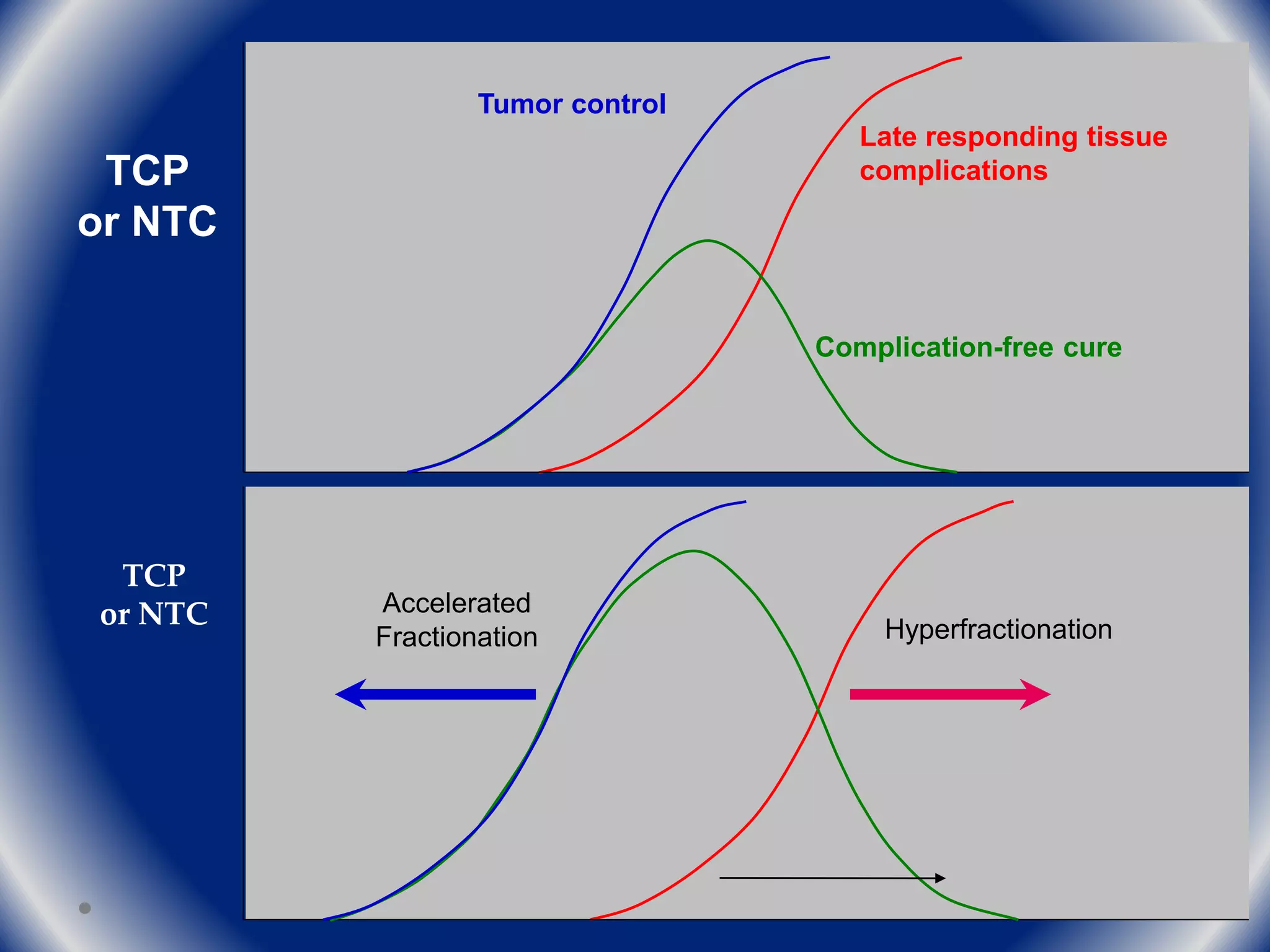
• If fractionation sensitivity of a cancer is similar to dose-limiting healthy
tissues, it may be possible to give fewer, larger fractions without
compromising effectiveness or safety](https://image.slidesharecdn.com/theradiobiologybehinddosefractionation-221118075212-57c26c7b/75/The-Radiobiology-Behind-Dose-Fractionation-pdf-41-2048.jpg)


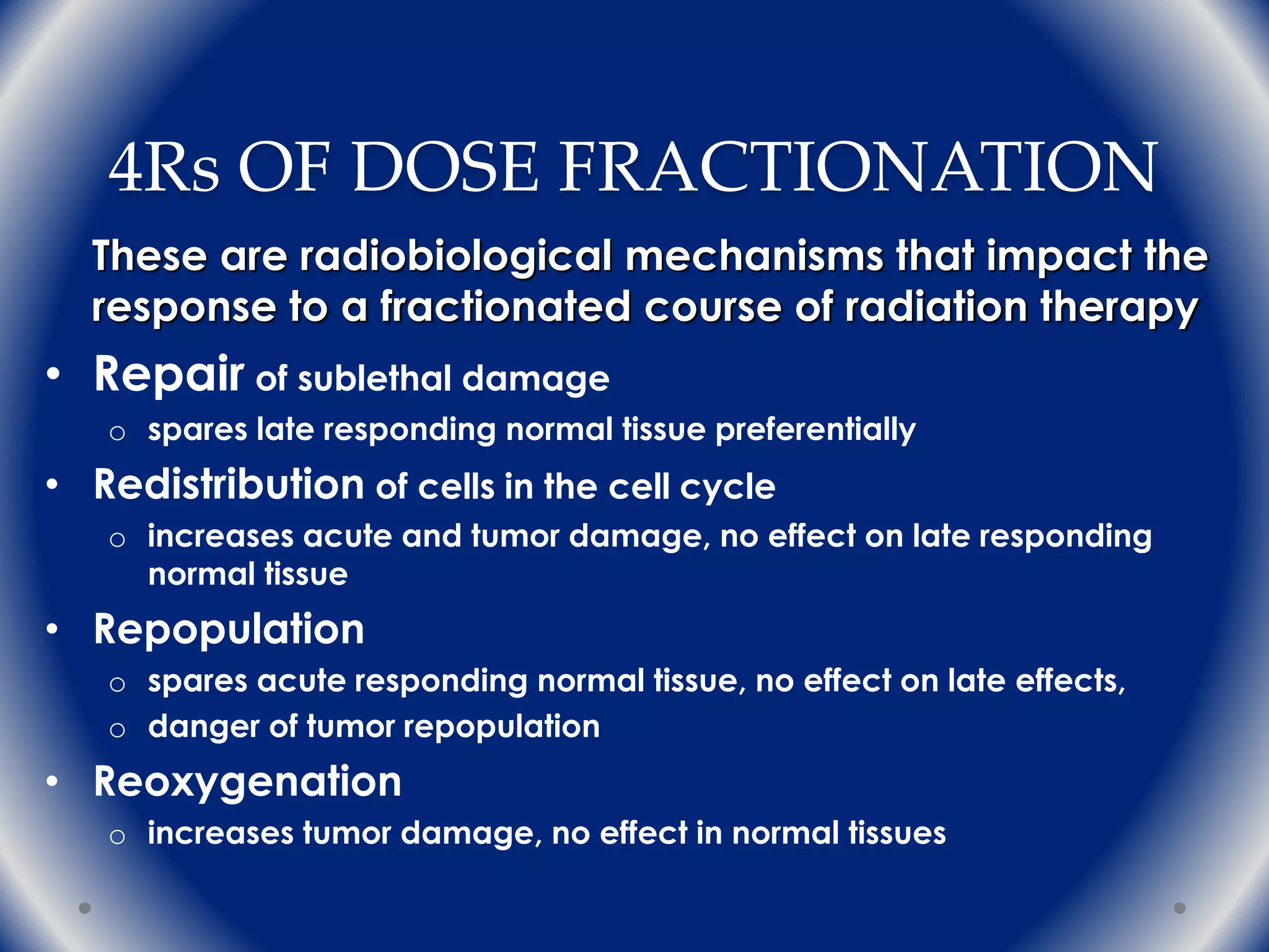
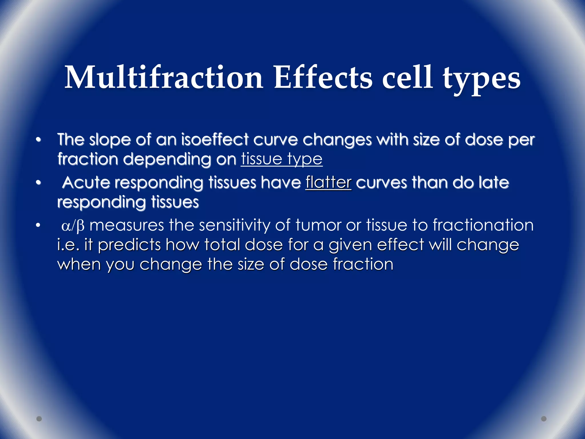
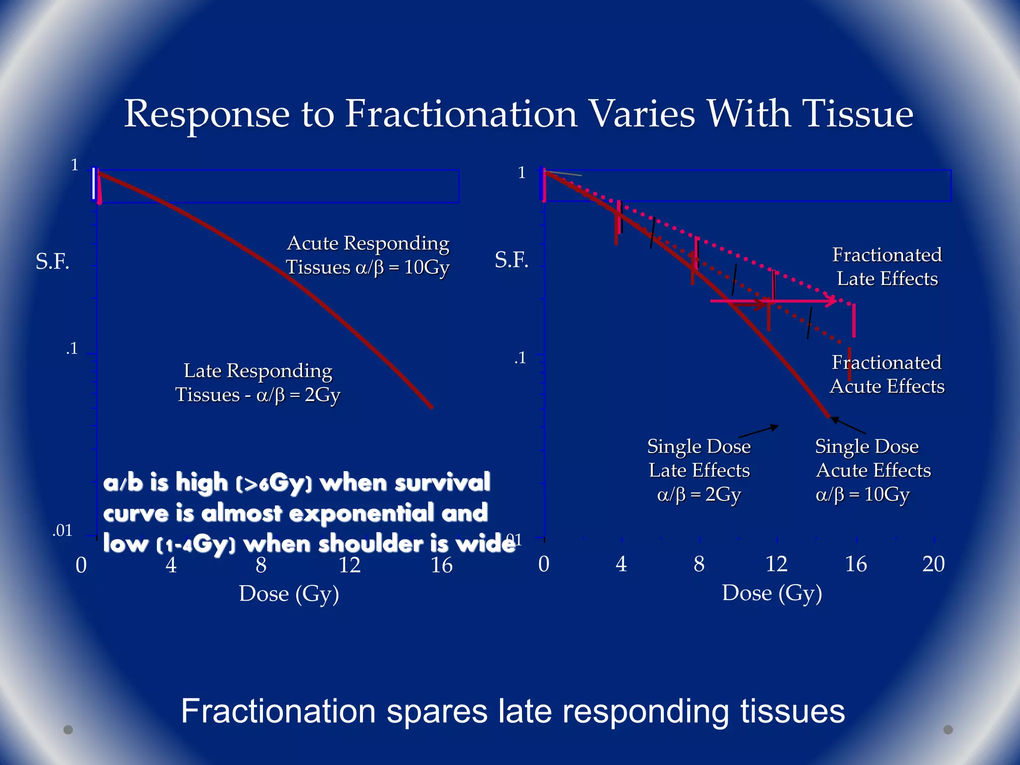
The document discusses the radiobiology principles underlying dose fractionation in radiation therapy, focusing on mathematical models like the linear quadratic model that describe cell survival curves and the impact of various fractionation schemes on tumor and normal tissue responses. It covers key concepts such as cell repair mechanisms, the 4Rs of radiobiology (repair, redistribution, repopulation, reoxygenation), and how different dose per fraction affect treatment outcomes. Additionally, it summarizes clinical trial findings on altered fractionation techniques and their implications for optimizing therapy to enhance tumor control while minimizing harm to healthy tissues.


![Arc therapy [autosaved] [autosaved]](https://cdn.slidesharecdn.com/ss_thumbnails/arctherapyautosavedautosaved-150423125828-conversion-gate01-thumbnail.jpg?width=640&height=640&fit=bounds)


