Downloaded 1,005 times


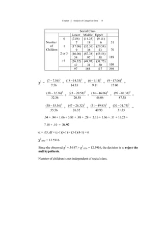


This document provides an overview and outline of Chapter 12 which covers the analysis of categorical data using two chi-square tests: the chi-square goodness-of-fit test and the chi-square test of independence. These tests are useful for analyzing nominal data, such as categories from market research, to determine if observed frequencies match expected distributions or if two variables are independent. The chapter also provides examples of solving problems using these tests and key terms related to categorical data analysis.


![Goodness of Fit [Autosaved] power point presentation](https://cdn.slidesharecdn.com/ss_thumbnails/goodnessoffitautosaved-241112161427-2da4f412-thumbnail.jpg?width=640&height=640&fit=bounds)


