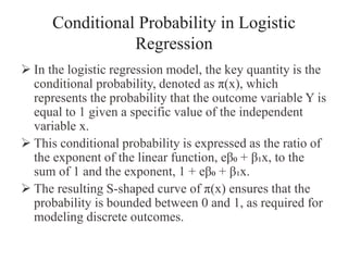
Conditional Probability in Logistic
Regression
 In the logistic regression model, the key quantity is the
conditional probability, denoted as π(x), which
represents the probability that the outcome variable Y is
equal to 1 given a specific value of the independent
variable x.
 This conditional probability is expressed as the ratio of
the exponent of the linear function, eβ₀ + β₁x, to the
sum of 1 and the exponent, 1 + eβ₀ + β₁x.
 The resulting S-shaped curve of π(x) ensures that the
probability is bounded between 0 and 1, as required for
modeling discrete outcomes.
It follows that the quantity 1 - π(x) gives the
conditional probability that Y is equal to 0 given
x, denoted as Pr(Y = 0|x).
For those pairs (xi, yi) where yi = 1, the
contribution to the likelihood function is π(xi),
and for those pairs where yi = 0, the contribution
is 1 - π(xi).
This formulation of the likelihood function based
on the conditional probabilities is a key aspect of
the maximum likelihood estimation approach
used in logistic regression analysis.
Maximum Likelihood Estimation
• The principle of maximum likelihood is central to the estimation of
the logistic regression model.
• The basic idea is to find the values of the unknown parameters, β₀
and β₁, that maximize the probability of observing the given set of
data.
• This is accomplished by constructing a likelihood function, which
expresses the probability of the observed data as a function of the
model parameters.
• The likelihood function for logistic regression is obtained as the
product of the terms representing the conditional probabilities of the
observed outcomes.
• Specifically, for each data point (x₋ᵢ, y₋ᵢ), where y₋ᵢ is the binary
outcome coded as 0 or 1, the contribution to the likelihood function
is π(x₋ᵢ)^y₋ᵢ * (1 - π(x₋ᵢ))^(1-y₋ᵢ).
• The full likelihood function is the product of these terms over all n
observations.
 To simplify the calculations, it is often more convenient
to work with the log of the likelihood function, known
as the log-likelihood.
 The maximum likelihood estimates of the parameters,
β₀ and β₁, are obtained by differentiating the log-
likelihood with respect to each parameter and setting
the resulting expressions equal to zero.
 These likelihood equations represent the conditions for
maximizing the likelihood function and provide a
systematic way to estimate the model parameters.
Solving Likelihood Equations
The solution to the likelihood equations can be
obtained using an iterative weighted least squares
procedure.
The values of β₀ and β₁ that satisfy these
equations are called the maximum likelihood
estimates and are denoted as β̂₀ and β̂₁,
respectively.
These estimates represent the values of the
parameters that maximize the likelihood function
and provide the best fit to the observed data.
 An interesting consequence of equation is that the sum of
the observed outcomes (y₁, y₂, ..., y_n) is equal to the sum
of the predicted probabilities (π̂(x₁), π̂(x₂), ..., π̂(x_n)).
 This means that the total number of observed "successes"
(y₁ = 1) is equal to the sum of the predicted probabilities
for each data point.
 This property is a useful diagnostic check for the validity
of the logistic regression model and the accuracy of the
maximum likelihood estimates.
Maximum Likelihood Estimates and Model
Fit
 Following the fitting of the logistic regression model, the
next step is to evaluate its adequacy and the statistical
significance of the estimated coefficients.
 The maximum likelihood estimates, denoted as β̂₀ and β̂₁,
provide the values of the parameters that maximize the
likelihood function and result in the best fit to the observed
data.
 These estimates can then be used to compute a variety of
diagnostic measures and test statistics to assess the overall
model fit and the individual effects of the independent
variables.
The logistic regression output typically includes
estimates of the standard errors of the
coefficients, the ratios of the estimated
coefficients to their standard errors (known as the
Wald statistics), and the corresponding p-values.
These quantities are essential for evaluating the
statistical significance of the independent
variables and determining which factors have a
meaningful impact on the outcome of interest.

conditional probablity in logistic regression

  • 1.
    Conditional Probability inLogistic Regression  In the logistic regression model, the key quantity is the conditional probability, denoted as π(x), which represents the probability that the outcome variable Y is equal to 1 given a specific value of the independent variable x.  This conditional probability is expressed as the ratio of the exponent of the linear function, eβ₀ + β₁x, to the sum of 1 and the exponent, 1 + eβ₀ + β₁x.  The resulting S-shaped curve of π(x) ensures that the probability is bounded between 0 and 1, as required for modeling discrete outcomes.
  • 2.
    It follows thatthe quantity 1 - π(x) gives the conditional probability that Y is equal to 0 given x, denoted as Pr(Y = 0|x). For those pairs (xi, yi) where yi = 1, the contribution to the likelihood function is π(xi), and for those pairs where yi = 0, the contribution is 1 - π(xi). This formulation of the likelihood function based on the conditional probabilities is a key aspect of the maximum likelihood estimation approach used in logistic regression analysis.
  • 3.
    Maximum Likelihood Estimation •The principle of maximum likelihood is central to the estimation of the logistic regression model. • The basic idea is to find the values of the unknown parameters, β₀ and β₁, that maximize the probability of observing the given set of data. • This is accomplished by constructing a likelihood function, which expresses the probability of the observed data as a function of the model parameters. • The likelihood function for logistic regression is obtained as the product of the terms representing the conditional probabilities of the observed outcomes. • Specifically, for each data point (x₋ᵢ, y₋ᵢ), where y₋ᵢ is the binary outcome coded as 0 or 1, the contribution to the likelihood function is π(x₋ᵢ)^y₋ᵢ * (1 - π(x₋ᵢ))^(1-y₋ᵢ). • The full likelihood function is the product of these terms over all n observations.
  • 4.
     To simplifythe calculations, it is often more convenient to work with the log of the likelihood function, known as the log-likelihood.  The maximum likelihood estimates of the parameters, β₀ and β₁, are obtained by differentiating the log- likelihood with respect to each parameter and setting the resulting expressions equal to zero.  These likelihood equations represent the conditions for maximizing the likelihood function and provide a systematic way to estimate the model parameters.
  • 5.
    Solving Likelihood Equations Thesolution to the likelihood equations can be obtained using an iterative weighted least squares procedure. The values of β₀ and β₁ that satisfy these equations are called the maximum likelihood estimates and are denoted as β̂₀ and β̂₁, respectively. These estimates represent the values of the parameters that maximize the likelihood function and provide the best fit to the observed data.
  • 6.
     An interestingconsequence of equation is that the sum of the observed outcomes (y₁, y₂, ..., y_n) is equal to the sum of the predicted probabilities (π̂(x₁), π̂(x₂), ..., π̂(x_n)).  This means that the total number of observed "successes" (y₁ = 1) is equal to the sum of the predicted probabilities for each data point.  This property is a useful diagnostic check for the validity of the logistic regression model and the accuracy of the maximum likelihood estimates.
  • 7.
    Maximum Likelihood Estimatesand Model Fit  Following the fitting of the logistic regression model, the next step is to evaluate its adequacy and the statistical significance of the estimated coefficients.  The maximum likelihood estimates, denoted as β̂₀ and β̂₁, provide the values of the parameters that maximize the likelihood function and result in the best fit to the observed data.  These estimates can then be used to compute a variety of diagnostic measures and test statistics to assess the overall model fit and the individual effects of the independent variables.
  • 8.
    The logistic regressionoutput typically includes estimates of the standard errors of the coefficients, the ratios of the estimated coefficients to their standard errors (known as the Wald statistics), and the corresponding p-values. These quantities are essential for evaluating the statistical significance of the independent variables and determining which factors have a meaningful impact on the outcome of interest.