Multivariable statistics_Using Stata

1. February 2025
ACIPH
Multivariable Analysis

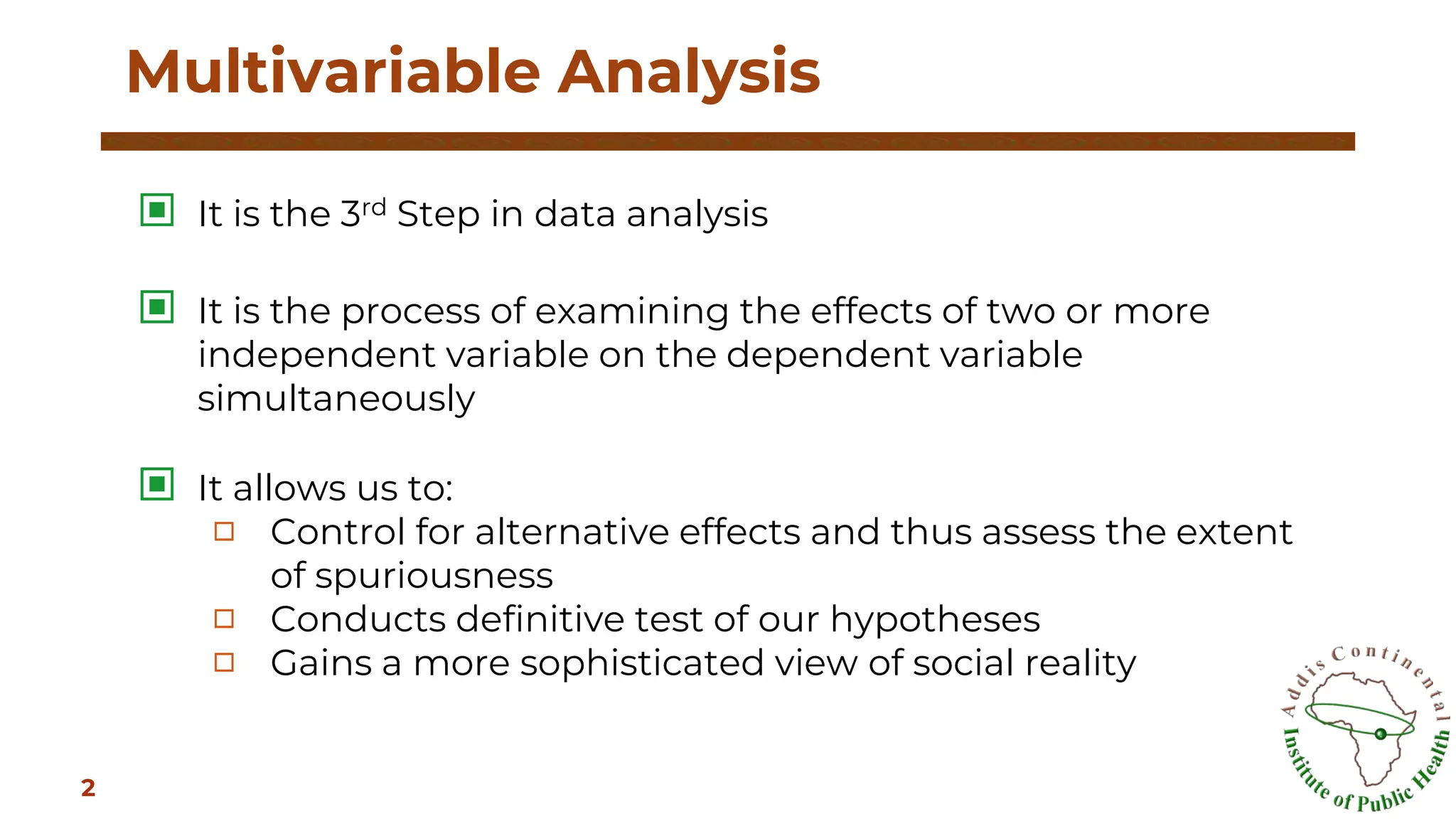
2. ▣ It is the 3rd Step in data analysis
▣ It is the process of examining the effects of two or more
independent variable on the dependent variable
simultaneously
▣ It allows us to:
□ Control for alternative effects and thus assess the extent
of spuriousness
□ Conducts definitive test of our hypotheses
□ Gains a more sophisticated view of social reality
Multivariable Analysis
2

3. Examples of Multivariable Analysis
3

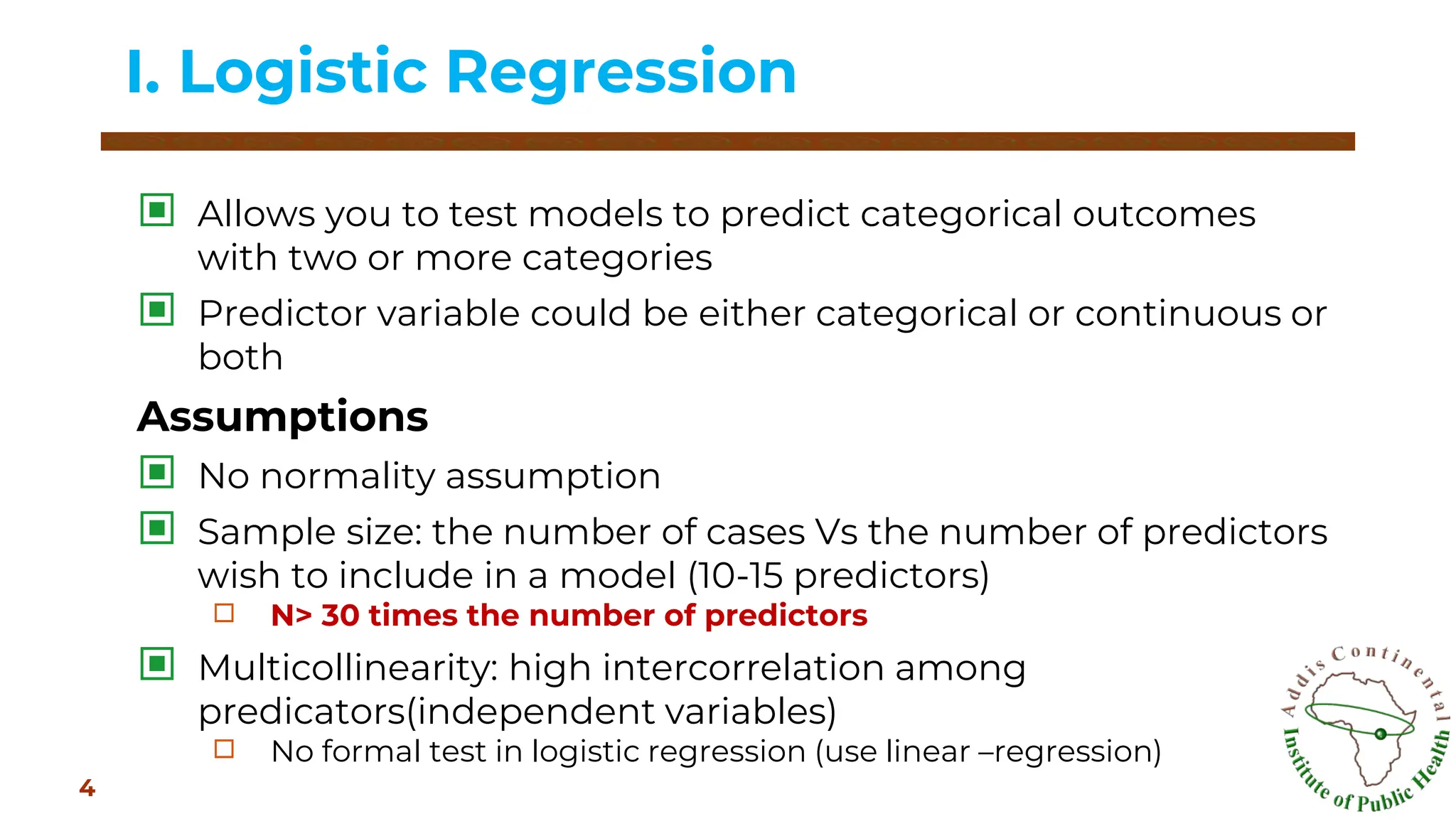
4. ▣ Allows you to test models to predict categorical outcomes
with two or more categories
▣ Predictor variable could be either categorical or continuous or
both
Assumptions
▣ No normality assumption
▣ Sample size: the number of cases Vs the number of predictors
wish to include in a model (10-15 predictors)
□ N> 30 times the number of predictors
▣ Multicollinearity: high intercorrelation among
predicators(independent variables)
□ No formal test in logistic regression (use linear –regression)
I. Logistic Regression
4

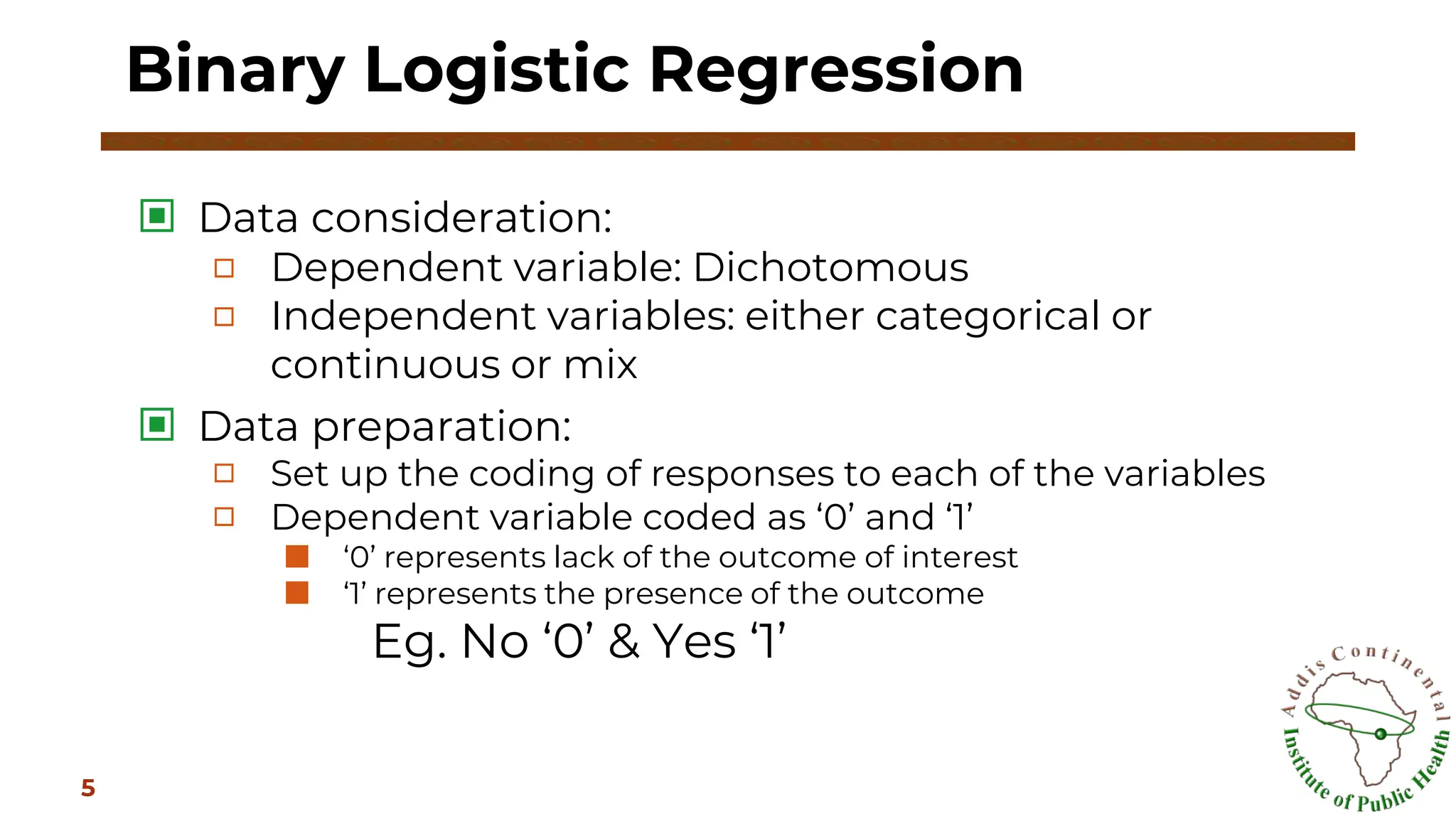
5. ▣ Data consideration:
□ Dependent variable: Dichotomous
□ Independent variables: either categorical or
continuous or mix
▣ Data preparation:
□ Set up the coding of responses to each of the variables
□ Dependent variable coded as ‘0’ and ‘1’
■ ‘0’ represents lack of the outcome of interest
■ ‘1’ represents the presence of the outcome
Eg. No ‘0’ & Yes ‘1’
Binary Logistic Regression
5

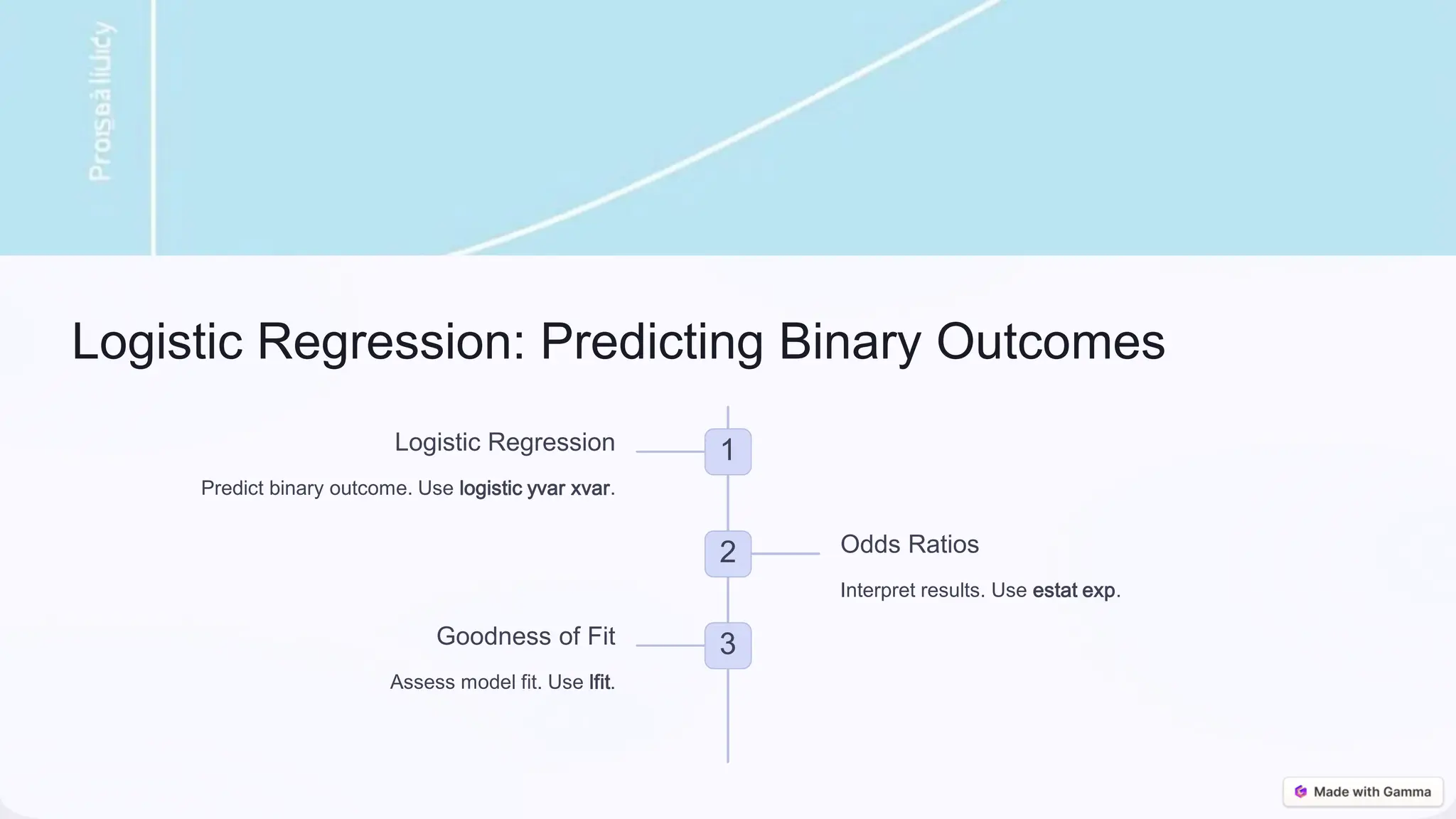
6. Logistic Regression: Predicting Binary Outcomes
1
Logistic Regression
Predict binary outcome. Use logistic yvar xvar.
2 Odds Ratios
Interpret results. Use estat exp.
3
Goodness of Fit
Assess model fit. Use lfit.

7. ▣ In the sample data set:
▣ Outcome variable: History of Myocardial
infarction
▣ Independent variables: Age category,
Gender, Physically active, Obesity, History of
diabetes, Blood pressure, Smoking,
Cholesterol, History of angina
Example
7

8. logit mi ib(first). agecat, or
Binary logistic regression Analysis
8

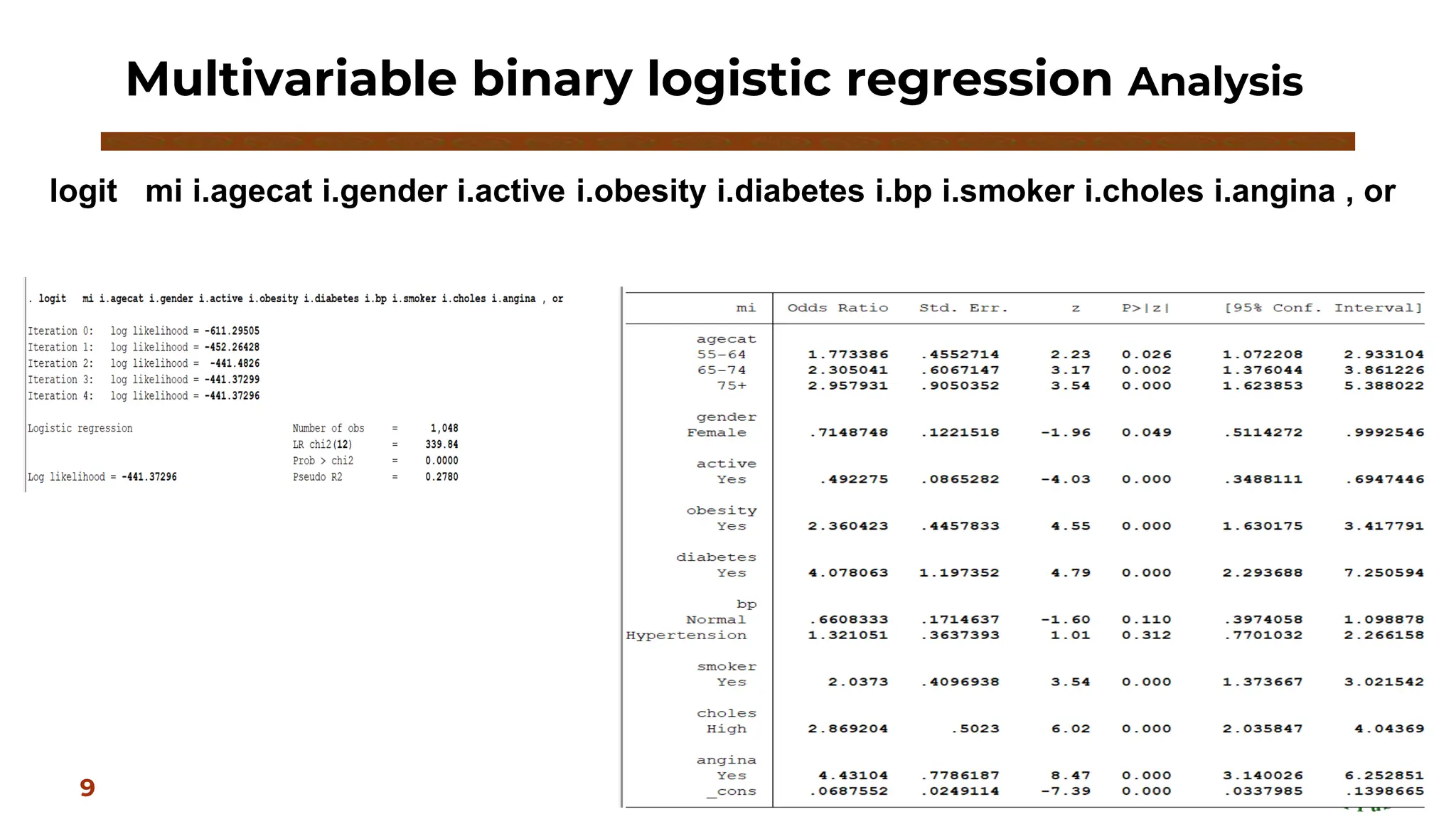
9. Multivariable binary logistic regression Analysis
9
logit mi i.agecat i.gender i.active i.obesity i.diabetes i.bp i.smoker i.choles i.angina , or

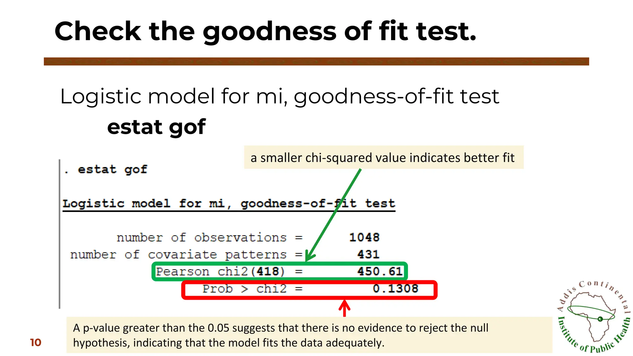
10. Logistic model for mi, goodness-of-fit test
estat gof
Check the goodness of fit test.
10
a smaller chi-squared value indicates better fit
A p-value greater than the 0.05 suggests that there is no evidence to reject the null
hypothesis, indicating that the model fits the data adequately.

11. ▣ How well are the independent variables
predict the outcome value
▣ Data considerations
□ The outcome variable must be continuous
□ The independent variables can be either
continuous or categorical
II. Multiple Linear Regression
11

12. ▪ Correlation seeks to establish whether a relationship exists
between two variables
▪ Regression seeks to use one variable to predict another
variable
▪ Both measure the extent of a linear relationship between two
variables
▪ Statistical tests are used to determine the strength of the
relationship
▪ A two-dimensional scatter plot is the fundamental graphical
tool for looking at regression and correlation data.
Overview of Correlation and Regression
12

13. ▪ Multicollinearity: high intercorrelation among
predicators(r=0.9 and above)
▪ Singularity: one independent variable is a
combination of other independent variables
▪ Outliers: very high or very low scores
▪ Delete it from the data
▪ Normality: the residuals should be normally
distributed about the predicted dependent variable
scores
Assumptions
13

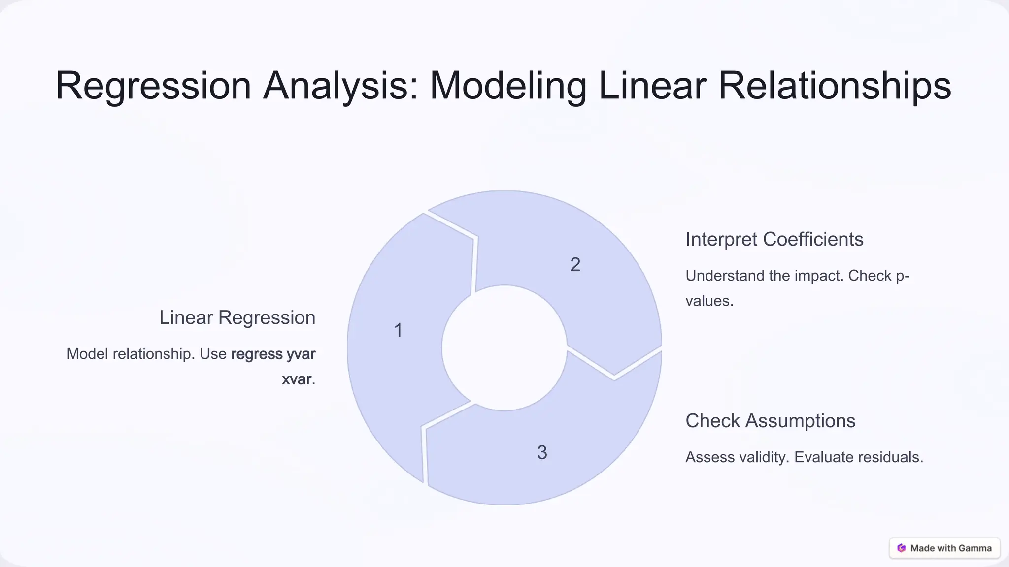
14. Regression Analysis: Modeling Linear Relationships
Linear Regression
Model relationship. Use regress yvar
xvar.
1
Interpret Coefficients
Understand the impact. Check p-
values.
2
Check Assumptions
Assess validity. Evaluate residuals.
3

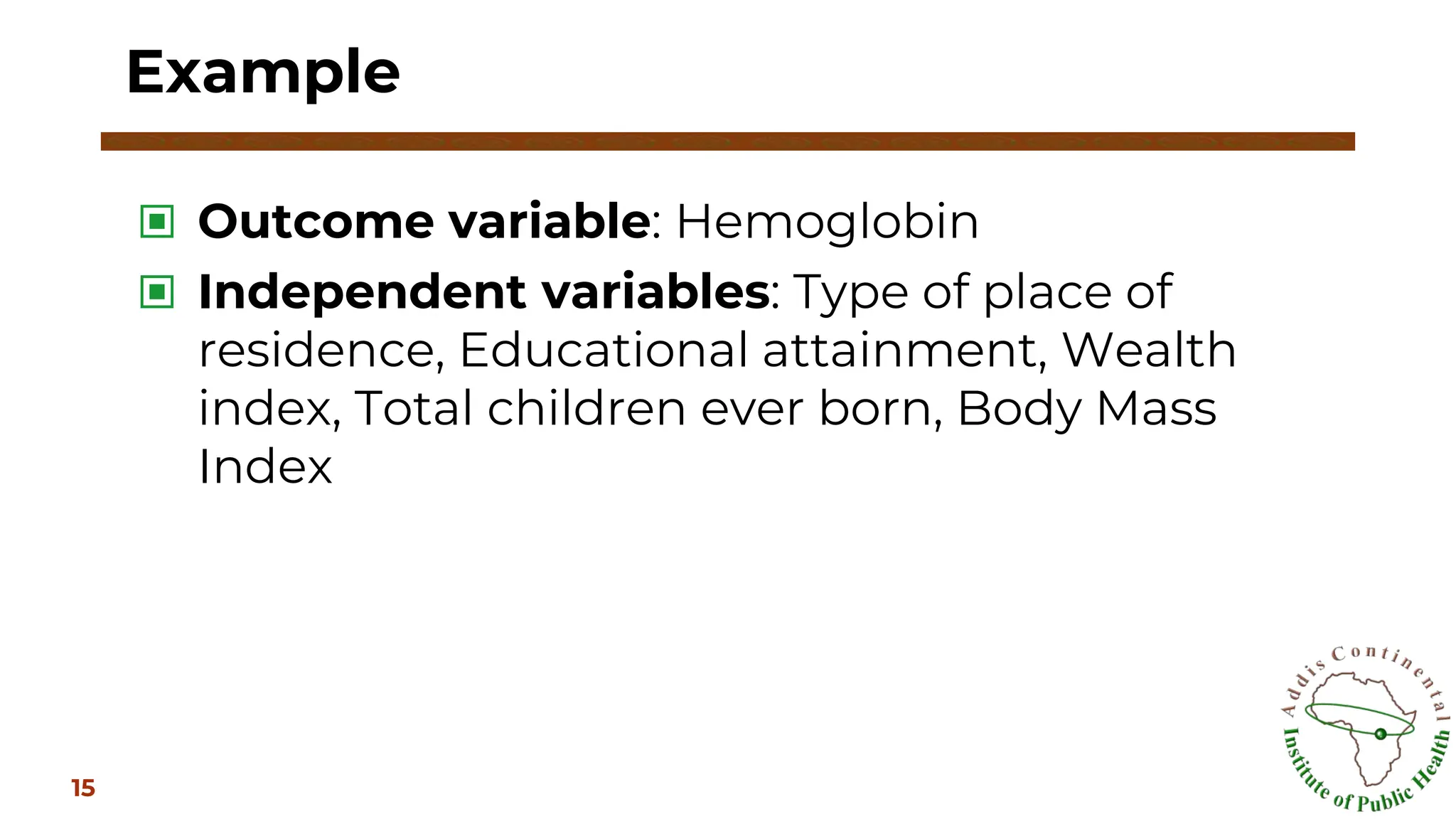
15. ▣ Outcome variable: Hemoglobin
▣ Independent variables: Type of place of
residence, Educational attainment, Wealth
index, Total children ever born, Body Mass
Index
Example
15

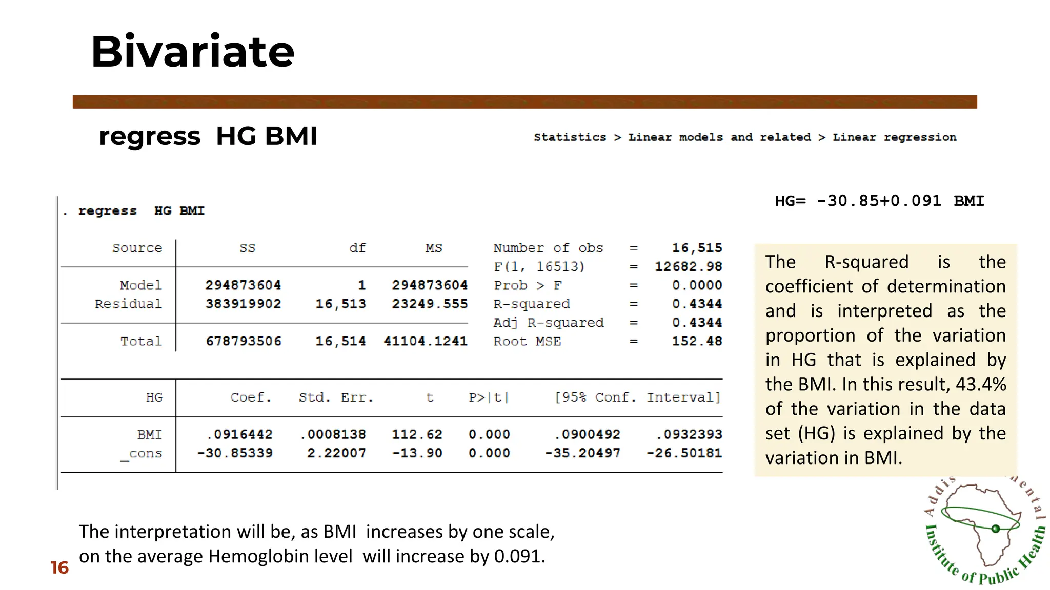
16. regress HG BMI
Bivariate
16
HG= -30.85+0.091 BMI
The interpretation will be, as BMI increases by one scale,
on the average Hemoglobin level will increase by 0.091.
The R-squared is the
coefficient of determination
and is interpreted as the
proportion of the variation
in HG that is explained by
the BMI. In this result, 43.4%
of the variation in the data
set (HG) is explained by the
variation in BMI.

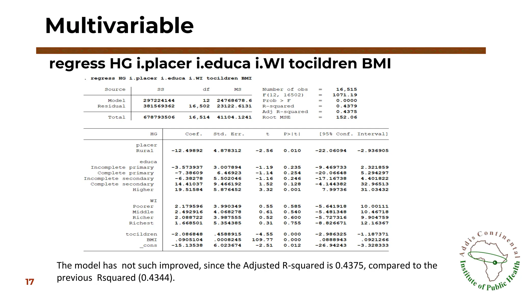
17. regress HG i.placer i.educa i.WI tocildren BMI
Multivariable
17
The model has not such improved, since the Adjusted R-squared is 0.4375, compared to the
previous Rsquared (0.4344).

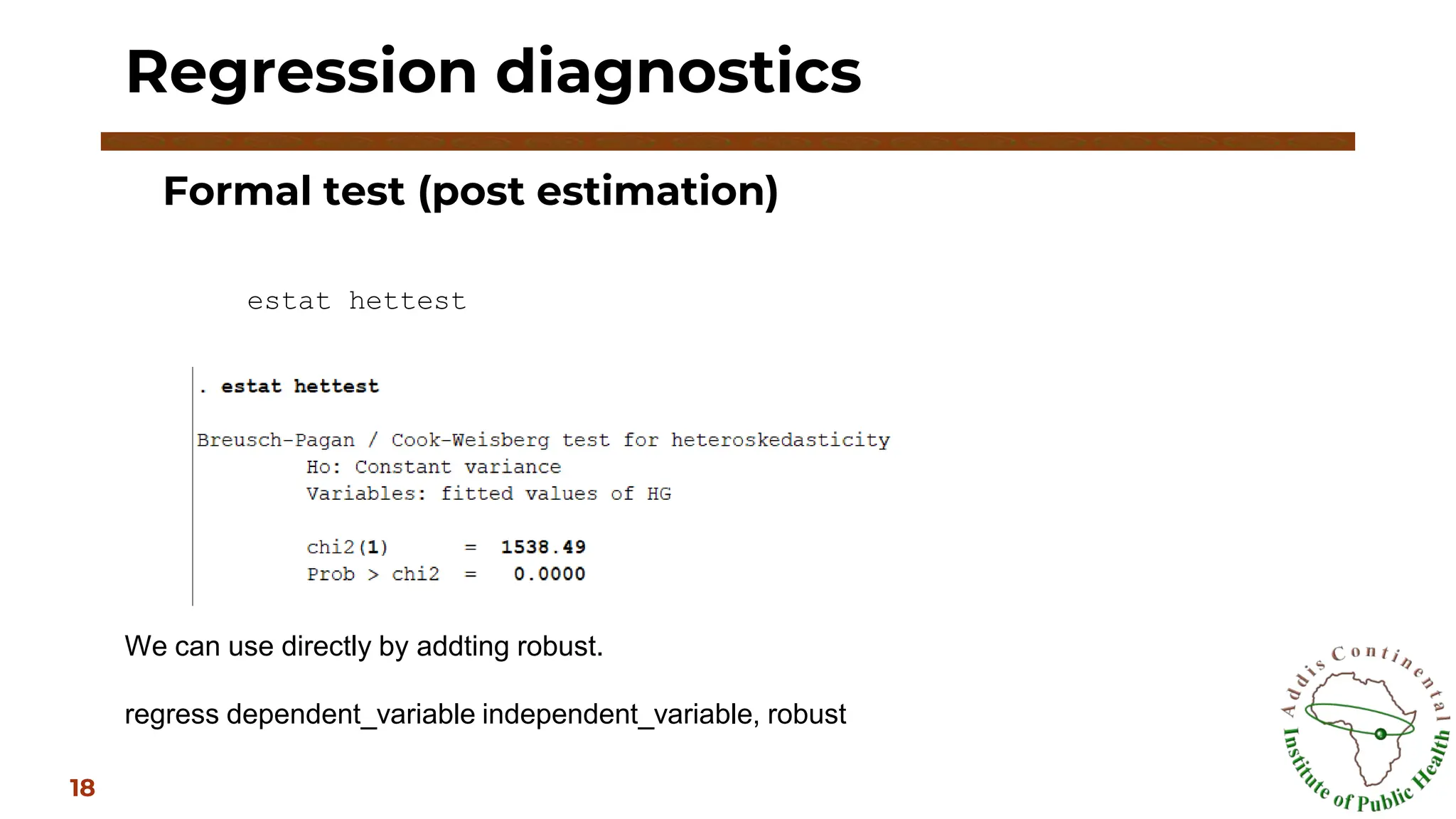
18. Formal test (post estimation)
Regression diagnostics
18
estat hettest
We can use directly by addting robust.
regress dependent_variable independent_variable, robust

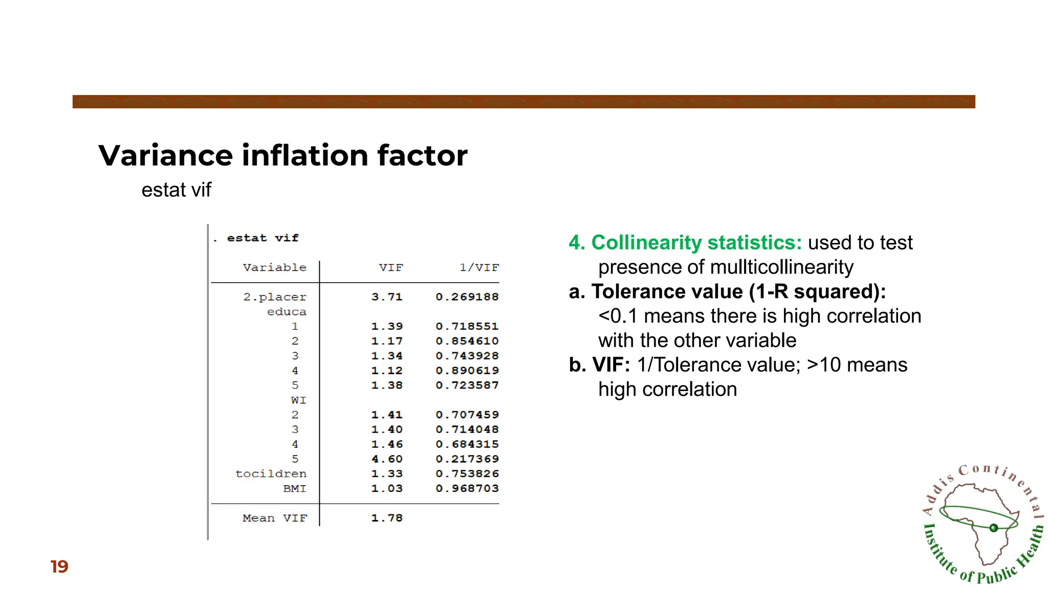
19. Variance inflation factor
19
estat vif
4. Collinearity statistics: used to test
presence of mullticollinearity
a. Tolerance value (1-R squared):
<0.1 means there is high correlation
with the other variable
b. VIF: 1/Tolerance value; >10 means
high correlation

20. ▪ ‘Survival’ means lack of experience of the event of
interest
▪ The word ‘survival’ does not necessary relate to lack of
death; it could mean failure to become diseased
▪ The generic name for the time is survival time,
▪ Statistical methods if the outcome of interest is time to
an event.
▪ In many medical studies, time to death is the event of
interest.
▪ Censoring and event are terminologies used in the
analysis
III. Survival analysis
20

21. ▣ Survival data are described in terms of two
probabilities, Hazard and Survival
▣ Survival is probability that an individual
survives from time origin (e.g. diagnosis of
cancer) to a specified future time.
▣ In contrast to the survival function, which
focuses on not having an event, the hazard
function focuses on the event occurring.
Hazard and survival
21

22. ▣ A person is counted as censored if he/she completed
the time of study with out the event or if he out-
migrated the study area before completing the study
▣ A person is counted as an event if he/she acquired the
event of interest
▣ All study subjects (both exposed/ unexposed) are
usually followed up till the end of study time to be
categorized to censored or event
Censoring and event
22

23. ▣ Life table method: a Method using probability
of occurrence during a range of time intervals
▣ Kaplan-meier method: it is a method that
depicts the probability of the event as the
event happens
▣ Cox-regression: it is similar to Kaplan-meier
method but using different categories as in a
regression during analysis
Three methods
23

24. ▪ We use intervals for the follow up time
▪ The length of time intervals used in the analysis is
somewhat arbitrary
▪ It should be selected so that the number of censored
observations in any interval is small
▪ Let us group by 1 year interval for the bednetstudy data
Life table method:
24

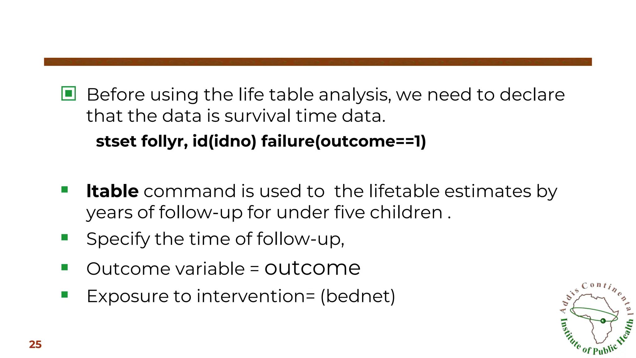
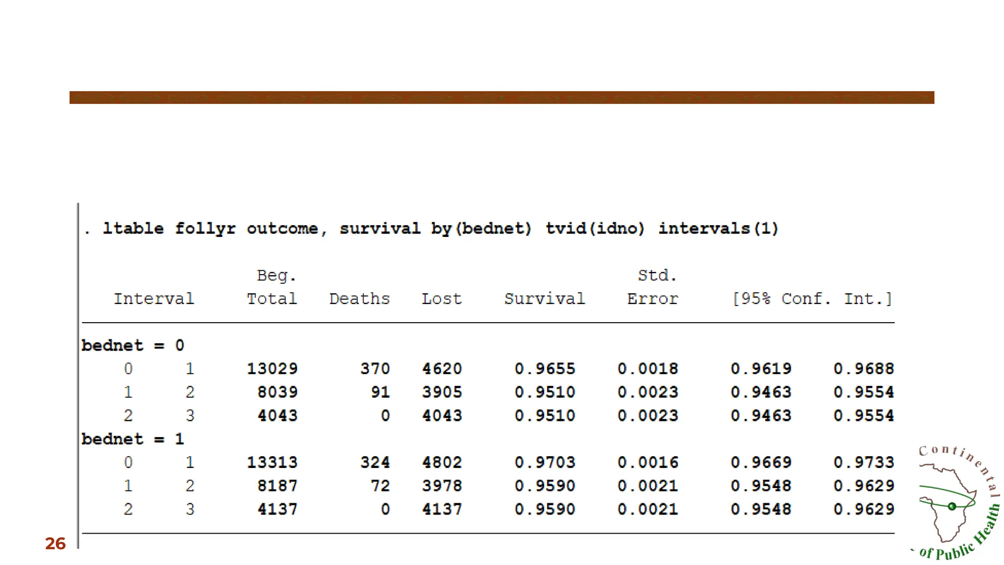
25. ▣ Before using the life table analysis, we need to declare
that the data is survival time data.
stset follyr, id(idno) failure(outcome==1)
▪ ltable command is used to the lifetable estimates by
years of follow-up for under five children .
▪ Specify the time of follow-up,
▪ Outcome variable = outcome
▪ Exposure to intervention= (bednet)
25

26. 26

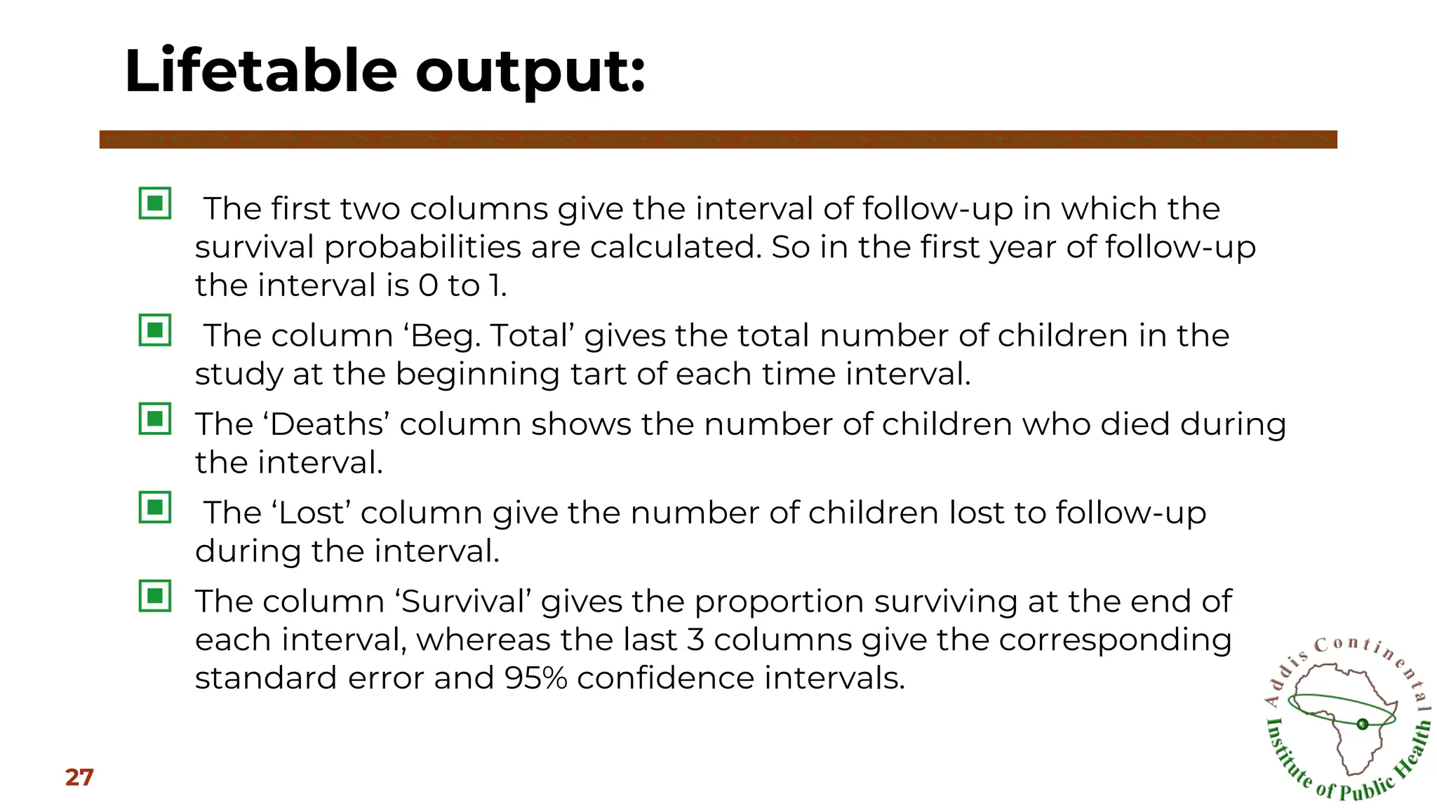
27. ▣ The first two columns give the interval of follow-up in which the
survival probabilities are calculated. So in the first year of follow-up
the interval is 0 to 1.
▣ The column ‘Beg. Total’ gives the total number of children in the
study at the beginning tart of each time interval.
▣ The ‘Deaths’ column shows the number of children who died during
the interval.
▣ The ‘Lost’ column give the number of children lost to follow-up
during the interval.
▣ The column ‘Survival’ gives the proportion surviving at the end of
each interval, whereas the last 3 columns give the corresponding
standard error and 95% confidence intervals.
Lifetable output:
27

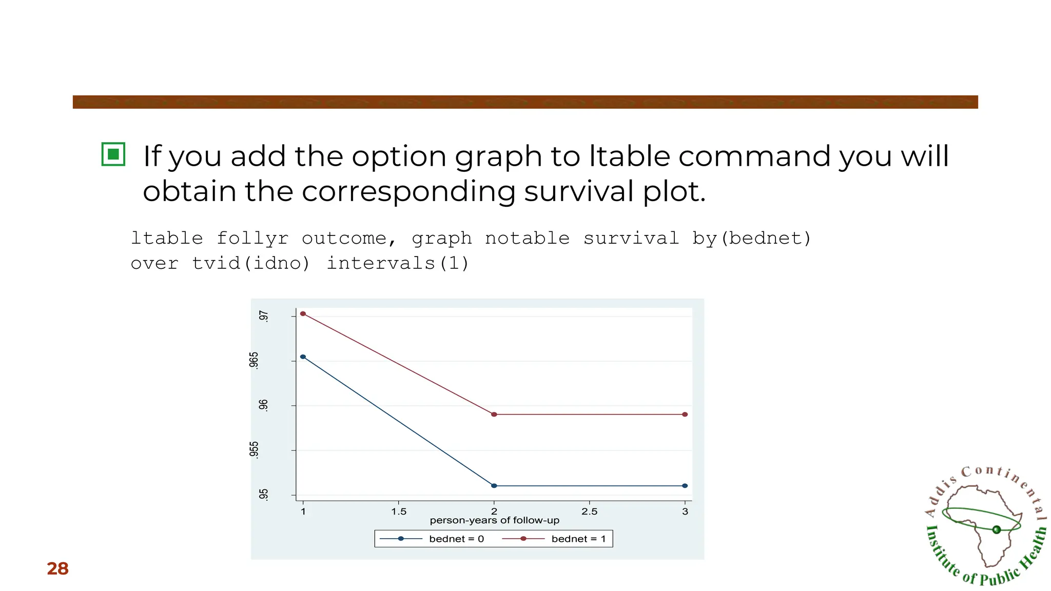
28. ▣ If you add the option graph to ltable command you will
obtain the corresponding survival plot.
28
ltable follyr outcome, graph notable survival by(bednet)
over tvid(idno) intervals(1)
.95
.955
.96
.965
.97
Proportion
Surviving
1 1.5 2 2.5 3
person-years of follow-up
bednet = 0 bednet = 1

29. ▪ Non-parametric estimate of the survival function:
o No math assumptions! (either about the underlying
hazard function or about proportional hazards).
o Simply, the empirical probability of surviving past
certain times in the sample (taking into account
censoring).
▪ Non-parametric estimate of the survival function.
o Commonly used to describe survivorship of study
population/s.
o Commonly used to compare two study populations.
Kaplan-meier method:
29

30. ▪ The Kaplan-Meier method of estimating survival is
similar to actuarial analysis except that time since entry
in the study is not divided into intervals for analysis.
▪ For this reason, it is especially appropriate in studies
involving a small number of patients.
▪ It involves fewer calculations than the actuarial method,
primarily because survival is estimated each time
outcome is occurred, so withdrawals are ignored.
30

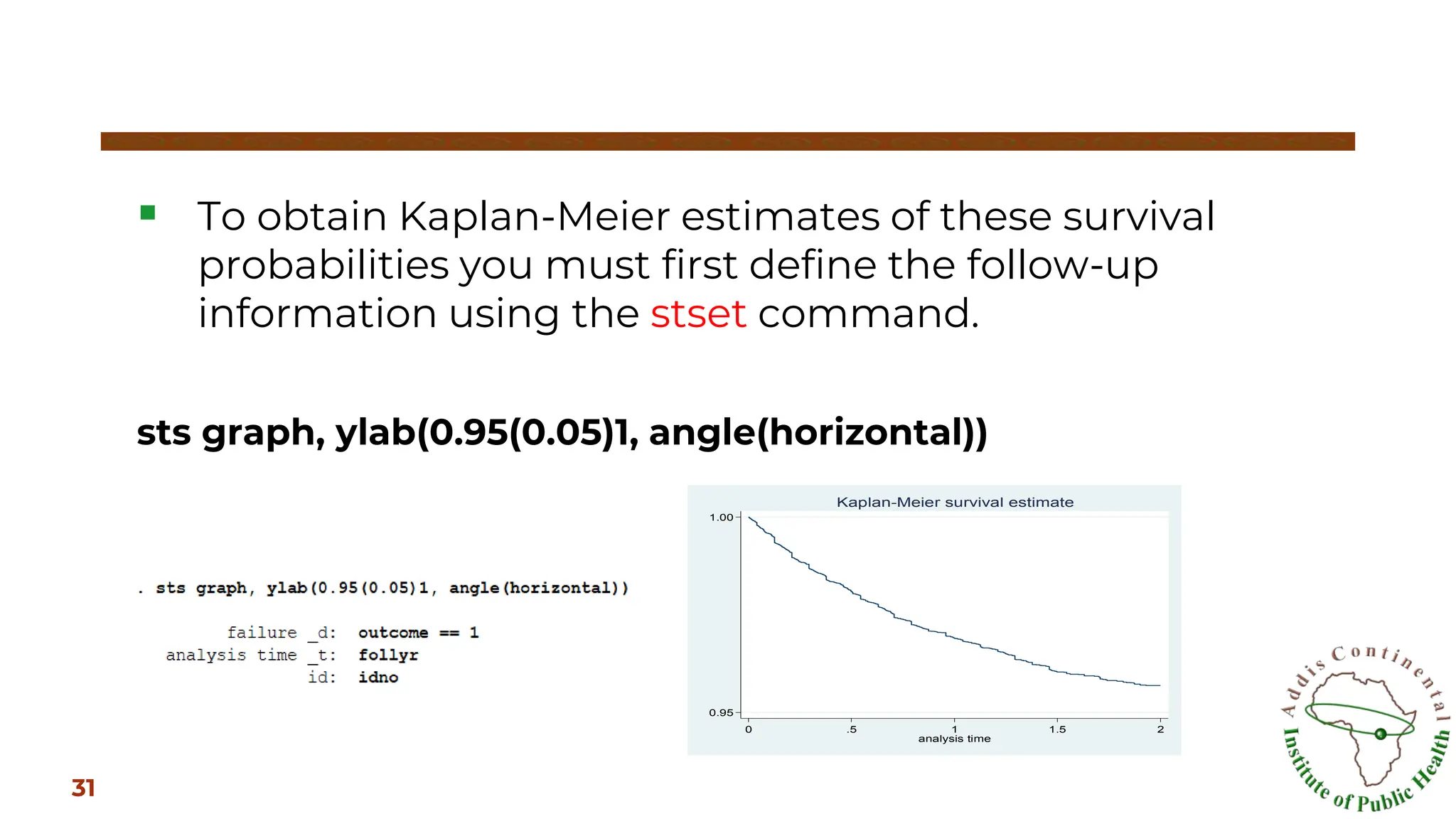
31. ▪ To obtain Kaplan-Meier estimates of these survival
probabilities you must first define the follow-up
information using the stset command.
sts graph, ylab(0.95(0.05)1, angle(horizontal))
31
0.95
1.00
0 .5 1 1.5 2
analysis time
Kaplan-Meier survival estimate

32. ▣ The Log-rank test compares the observed and expected
distribution of events between two or more groups.
▣ For example, we can compared the survival time between
those exposed to the intervention and the control group.
▣ In the logrank test, we compare the number of observed
failures in each group with the number of failures that would
be expected from the losses in the combined groups, i.e., if
group membership did not matter.
▣ Log-rank test is just a Cochran-Mantel-Haenszel chi-square
test!
sts test bednet, logrank
Log-rank Test:
32

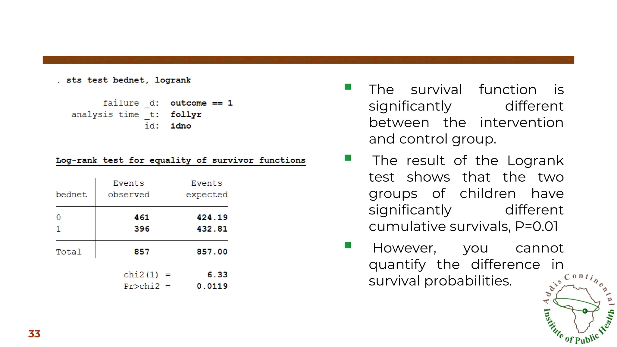
33. ▪ The survival function is
significantly different
between the intervention
and control group.
▪ The result of the Logrank
test shows that the two
groups of children have
significantly different
cumulative survivals, P=0.01
▪ However, you cannot
quantify the difference in
survival probabilities.
33

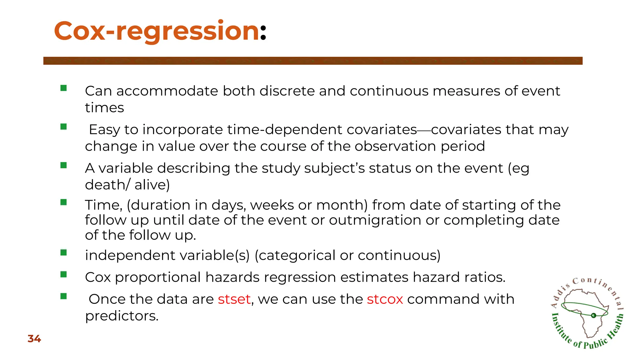
34. ▪ Can accommodate both discrete and continuous measures of event
times
▪ Easy to incorporate time-dependent covariates—covariates that may
change in value over the course of the observation period
▪ A variable describing the study subject’s status on the event (eg
death/ alive)
▪ Time, (duration in days, weeks or month) from date of starting of the
follow up until date of the event or outmigration or completing date
of the follow up.
▪ independent variable(s) (categorical or continuous)
▪ Cox proportional hazards regression estimates hazard ratios.
▪ Once the data are stset, we can use the stcox command with
predictors.
Cox-regression:
34

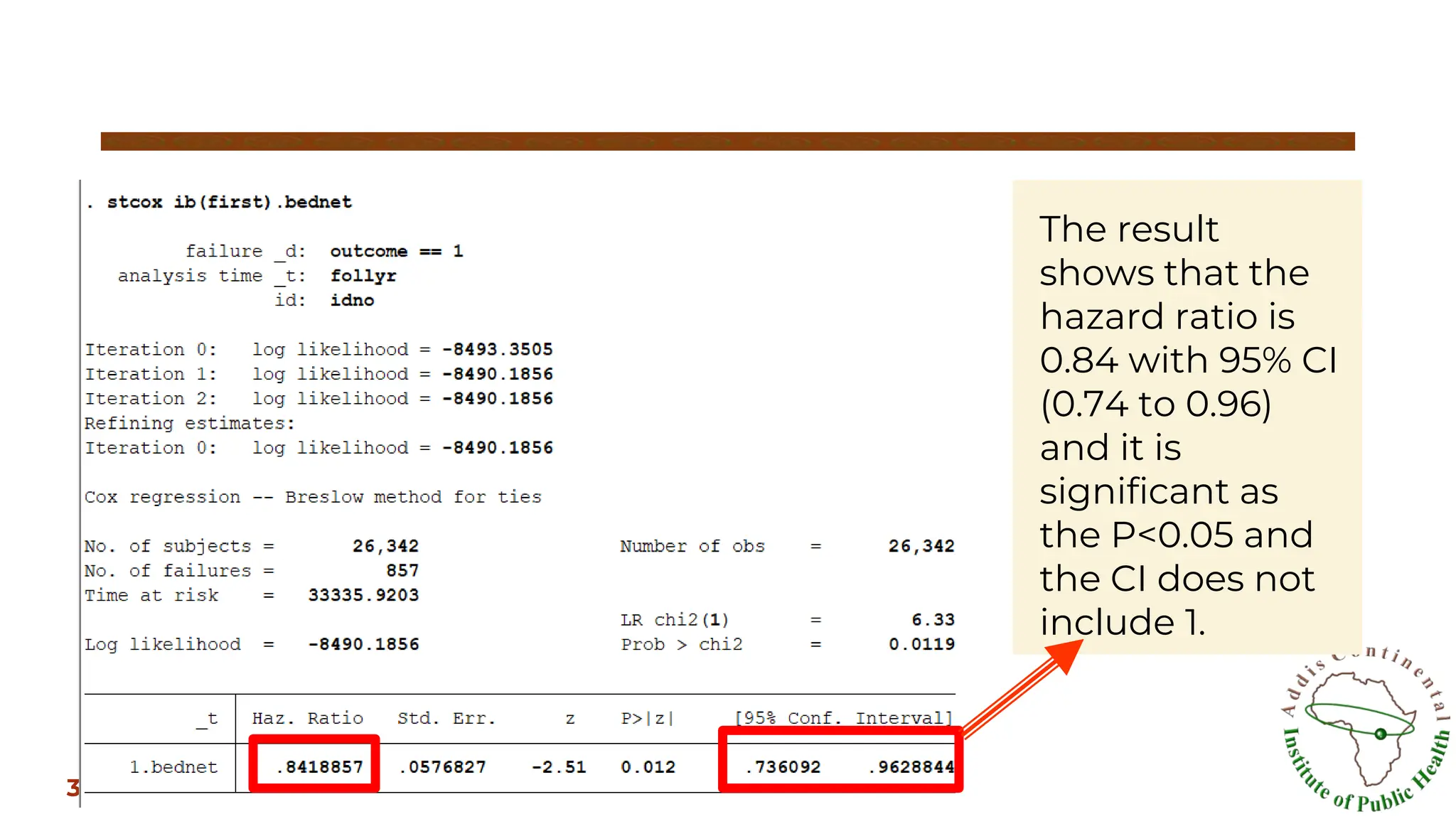
35. The result
shows that the
hazard ratio is
0.84 with 95% CI
(0.74 to 0.96)
and it is
significant as
the P<0.05 and
the CI does not
include 1.
35

36. Multivariate analysis
36
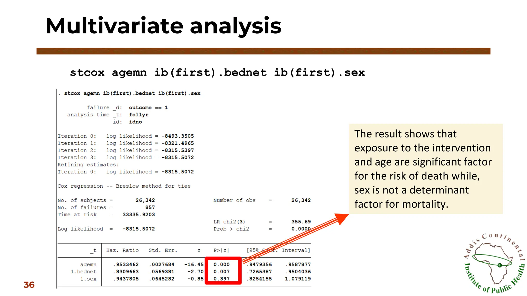
stcox agemn ib(first).bednet ib(first).sex
The result shows that
exposure to the intervention
and age are significant factor
for the risk of death while,
sex is not a determinant
factor for mortality.

37. Thank you!
37