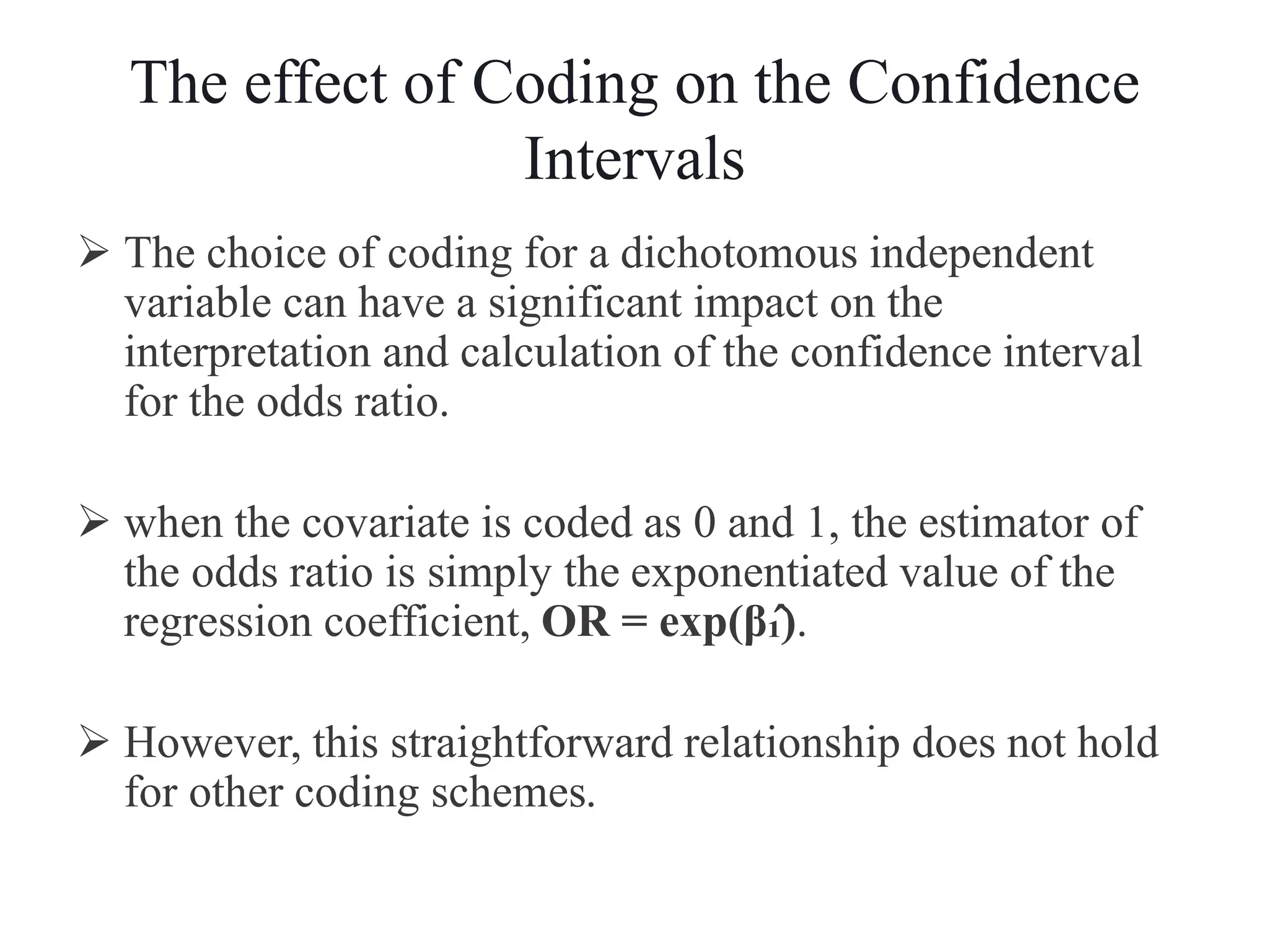
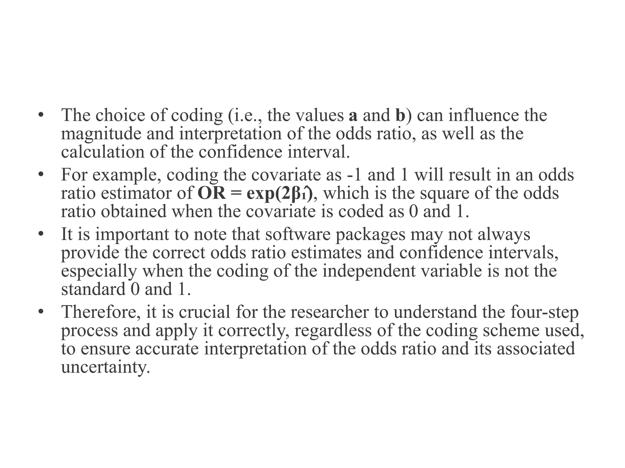
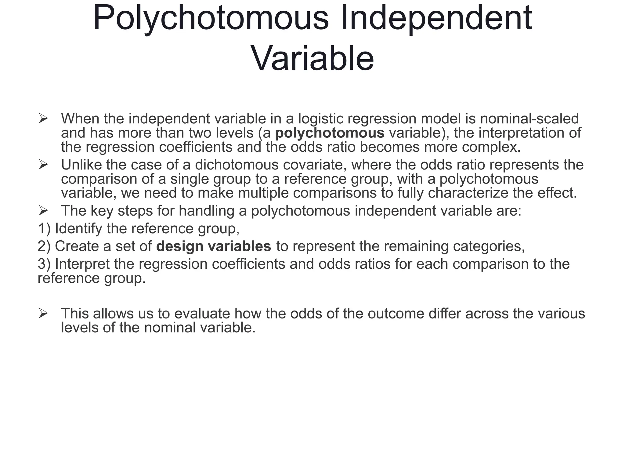
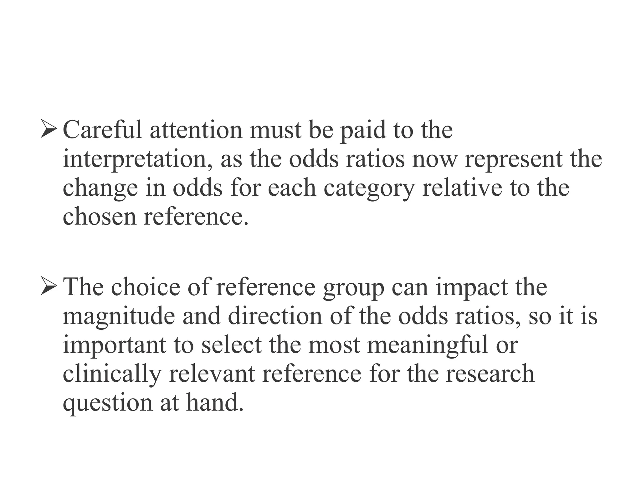
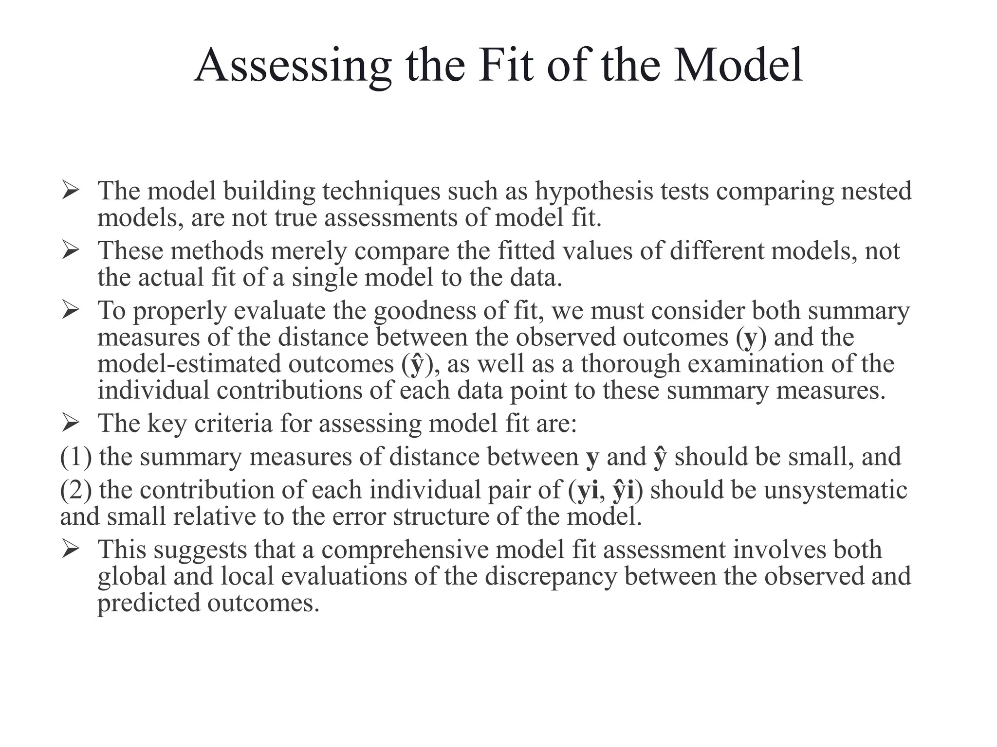
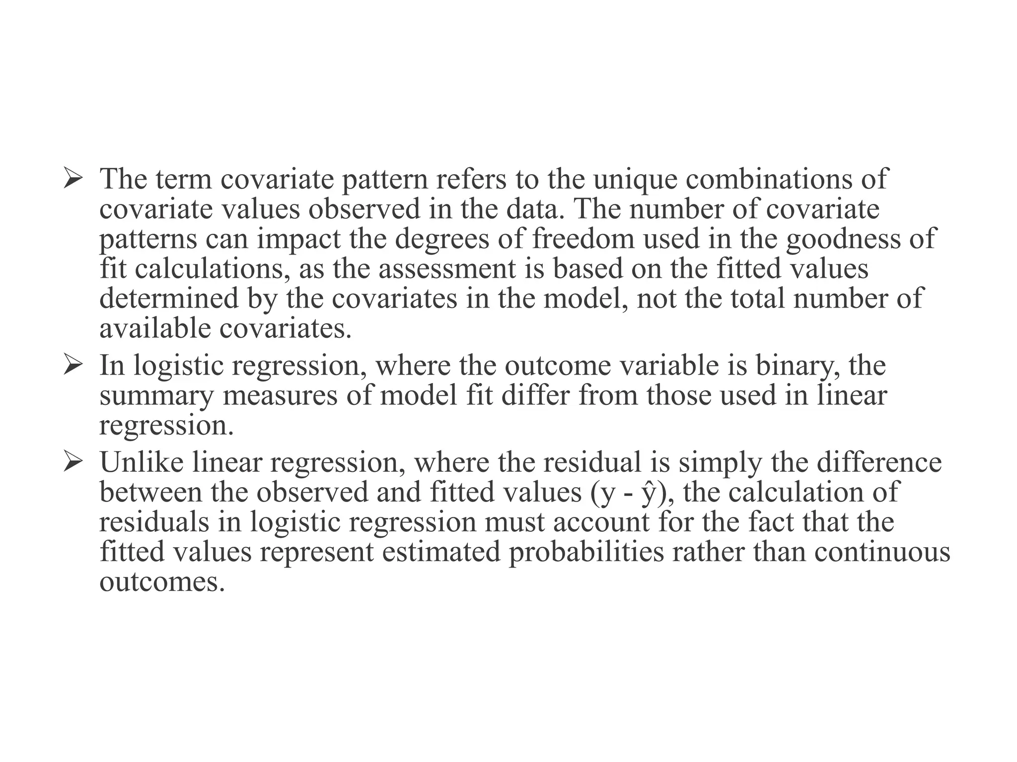
The effect of Coding on the Confidence
Intervals
 The choice of coding for a dichotomous independent
variable can have a significant impact on the
interpretation and calculation of the confidence interval
for the odds ratio.
 when the covariate is coded as 0 and 1, the estimator of
the odds ratio is simply the exponentiated value of the
regression coefficient, OR = exp(β₁̂).
 However, this straightforward relationship does not hold
for other coding schemes.
• The choice of coding (i.e., the values a and b) can influence the
magnitude and interpretation of the odds ratio, as well as the
calculation of the confidence interval.
• For example, coding the covariate as -1 and 1 will result in an odds
ratio estimator of OR = exp(2β₁̂), which is the square of the odds
ratio obtained when the covariate is coded as 0 and 1.
• It is important to note that software packages may not always
provide the correct odds ratio estimates and confidence intervals,
especially when the coding of the independent variable is not the
standard 0 and 1.
• Therefore, it is crucial for the researcher to understand the four-step
process and apply it correctly, regardless of the coding scheme used,
to ensure accurate interpretation of the odds ratio and its associated
uncertainty.
Polychotomous Independent
Variable
 When the independent variable in a logistic regression model is nominal-scaled
and has more than two levels (a polychotomous variable), the interpretation of
the regression coefficients and the odds ratio becomes more complex.
 Unlike the case of a dichotomous covariate, where the odds ratio represents the
comparison of a single group to a reference group, with a polychotomous
variable, we need to make multiple comparisons to fully characterize the effect.
 The key steps for handling a polychotomous independent variable are:
1) Identify the reference group,
2) Create a set of design variables to represent the remaining categories,
3) Interpret the regression coefficients and odds ratios for each comparison to the
reference group.
 This allows us to evaluate how the odds of the outcome differ across the various
levels of the nominal variable.
Careful attention must be paid to the
interpretation, as the odds ratios now represent the
change in odds for each category relative to the
chosen reference.
The choice of reference group can impact the
magnitude and direction of the odds ratios, so it is
important to select the most meaningful or
clinically relevant reference for the research
question at hand.
Assessing the Fit of the Model
 The model building techniques such as hypothesis tests comparing nested
models, are not true assessments of model fit.
 These methods merely compare the fitted values of different models, not
the actual fit of a single model to the data.
 To properly evaluate the goodness of fit, we must consider both summary
measures of the distance between the observed outcomes (y) and the
model-estimated outcomes (ŷ), as well as a thorough examination of the
individual contributions of each data point to these summary measures.
 The key criteria for assessing model fit are:
(1) the summary measures of distance between y and ŷ should be small, and
(2) the contribution of each individual pair of (yi, ŷi) should be unsystematic
and small relative to the error structure of the model.
 This suggests that a comprehensive model fit assessment involves both
global and local evaluations of the discrepancy between the observed and
predicted outcomes.
Model Fit Assessment Techniques
The key components of a comprehensive
model fit assessment approach are:
-Computation and evaluation of overall measures of fit,
such as the Pearson Chi-Square statistic, deviance, or sum-
of-squares, which provide a global indication of how well
the model fits the data.
- Examination of the individual components of the
summary statistics, often through graphical techniques,
to identify any systematic patterns or outliers that may
indicate areas where the model is not adequately fitting
the data.
- Comparison of the observed and fitted values, not in
relation to a smaller model, but in an absolute sense,
considering the fitted model as a representation of the best
possible (saturated) model.
Measures of Goodness of Fit
 When assessing the fit of a model, it is important to
consider various summary measures of goodness of fit.
 These statistics provide a global indication of how well the
model fits the data, but they do not necessarily reveal
information about the individual contributions of each data
point.
 While a small value for these measures can be a good sign,
it does not rule out the possibility of substantial deviations
from fit for some observations. Conversely, a large value is
a clear indication that the model is not adequately capturing
the underlying relationships in the data.
 An important consideration when using these summary
measures is the effect the fitted model has on the degrees of
freedom available for the assessment.
 The term covariate pattern refers to the unique combinations of
covariate values observed in the data. The number of covariate
patterns can impact the degrees of freedom used in the goodness of
fit calculations, as the assessment is based on the fitted values
determined by the covariates in the model, not the total number of
available covariates.
 In logistic regression, where the outcome variable is binary, the
summary measures of model fit differ from those used in linear
regression.
 Unlike linear regression, where the residual is simply the difference
between the observed and fitted values (y - ŷ), the calculation of
residuals in logistic regression must account for the fact that the
fitted values represent estimated probabilities rather than continuous
outcomes.
 The three key summary measures used to assess the goodness of fit
in logistic regression are the Pearson Chi-Square statistic, the
deviance, and the sum-of-squares.
 For a particular covariate pattern j, the Pearson residual is
calculated as:
r(yj, π̂j) = (yj - mjπ̂j) / √(mjπ̂j(1 - π̂j))
 The Pearson Chi-Square statistic is then the sum of the squares of
these Pearson residuals across all covariate patterns:
X2 = Σj=1J [r(yj, π̂j)]2
 The deviance residual and the sum-of-squares residual are two
alternative measures that also capture the discrepancy between the
observed and fitted values. These summary statistics, when
considered alongside the examination of individual residuals,
provide a comprehensive assessment of the model's goodness of fit.

binary logistic assessment methods and strategies

  • 1.
    The effect ofCoding on the Confidence Intervals  The choice of coding for a dichotomous independent variable can have a significant impact on the interpretation and calculation of the confidence interval for the odds ratio.  when the covariate is coded as 0 and 1, the estimator of the odds ratio is simply the exponentiated value of the regression coefficient, OR = exp(β₁̂).  However, this straightforward relationship does not hold for other coding schemes.
  • 2.
    • The choiceof coding (i.e., the values a and b) can influence the magnitude and interpretation of the odds ratio, as well as the calculation of the confidence interval. • For example, coding the covariate as -1 and 1 will result in an odds ratio estimator of OR = exp(2β₁̂), which is the square of the odds ratio obtained when the covariate is coded as 0 and 1. • It is important to note that software packages may not always provide the correct odds ratio estimates and confidence intervals, especially when the coding of the independent variable is not the standard 0 and 1. • Therefore, it is crucial for the researcher to understand the four-step process and apply it correctly, regardless of the coding scheme used, to ensure accurate interpretation of the odds ratio and its associated uncertainty.
  • 3.
    Polychotomous Independent Variable  Whenthe independent variable in a logistic regression model is nominal-scaled and has more than two levels (a polychotomous variable), the interpretation of the regression coefficients and the odds ratio becomes more complex.  Unlike the case of a dichotomous covariate, where the odds ratio represents the comparison of a single group to a reference group, with a polychotomous variable, we need to make multiple comparisons to fully characterize the effect.  The key steps for handling a polychotomous independent variable are: 1) Identify the reference group, 2) Create a set of design variables to represent the remaining categories, 3) Interpret the regression coefficients and odds ratios for each comparison to the reference group.  This allows us to evaluate how the odds of the outcome differ across the various levels of the nominal variable.
  • 4.
    Careful attention mustbe paid to the interpretation, as the odds ratios now represent the change in odds for each category relative to the chosen reference. The choice of reference group can impact the magnitude and direction of the odds ratios, so it is important to select the most meaningful or clinically relevant reference for the research question at hand.
  • 5.
    Assessing the Fitof the Model  The model building techniques such as hypothesis tests comparing nested models, are not true assessments of model fit.  These methods merely compare the fitted values of different models, not the actual fit of a single model to the data.  To properly evaluate the goodness of fit, we must consider both summary measures of the distance between the observed outcomes (y) and the model-estimated outcomes (ŷ), as well as a thorough examination of the individual contributions of each data point to these summary measures.  The key criteria for assessing model fit are: (1) the summary measures of distance between y and ŷ should be small, and (2) the contribution of each individual pair of (yi, ŷi) should be unsystematic and small relative to the error structure of the model.  This suggests that a comprehensive model fit assessment involves both global and local evaluations of the discrepancy between the observed and predicted outcomes.
  • 6.
    Model Fit AssessmentTechniques The key components of a comprehensive model fit assessment approach are: -Computation and evaluation of overall measures of fit, such as the Pearson Chi-Square statistic, deviance, or sum- of-squares, which provide a global indication of how well the model fits the data.
  • 7.
    - Examination ofthe individual components of the summary statistics, often through graphical techniques, to identify any systematic patterns or outliers that may indicate areas where the model is not adequately fitting the data. - Comparison of the observed and fitted values, not in relation to a smaller model, but in an absolute sense, considering the fitted model as a representation of the best possible (saturated) model.
  • 8.
    Measures of Goodnessof Fit  When assessing the fit of a model, it is important to consider various summary measures of goodness of fit.  These statistics provide a global indication of how well the model fits the data, but they do not necessarily reveal information about the individual contributions of each data point.  While a small value for these measures can be a good sign, it does not rule out the possibility of substantial deviations from fit for some observations. Conversely, a large value is a clear indication that the model is not adequately capturing the underlying relationships in the data.  An important consideration when using these summary measures is the effect the fitted model has on the degrees of freedom available for the assessment.
  • 9.
     The termcovariate pattern refers to the unique combinations of covariate values observed in the data. The number of covariate patterns can impact the degrees of freedom used in the goodness of fit calculations, as the assessment is based on the fitted values determined by the covariates in the model, not the total number of available covariates.  In logistic regression, where the outcome variable is binary, the summary measures of model fit differ from those used in linear regression.  Unlike linear regression, where the residual is simply the difference between the observed and fitted values (y - ŷ), the calculation of residuals in logistic regression must account for the fact that the fitted values represent estimated probabilities rather than continuous outcomes.
  • 10.
     The threekey summary measures used to assess the goodness of fit in logistic regression are the Pearson Chi-Square statistic, the deviance, and the sum-of-squares.  For a particular covariate pattern j, the Pearson residual is calculated as: r(yj, π̂j) = (yj - mjπ̂j) / √(mjπ̂j(1 - π̂j))  The Pearson Chi-Square statistic is then the sum of the squares of these Pearson residuals across all covariate patterns: X2 = Σj=1J [r(yj, π̂j)]2  The deviance residual and the sum-of-squares residual are two alternative measures that also capture the discrepancy between the observed and fitted values. These summary statistics, when considered alongside the examination of individual residuals, provide a comprehensive assessment of the model's goodness of fit.