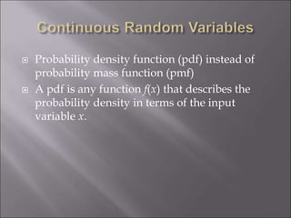
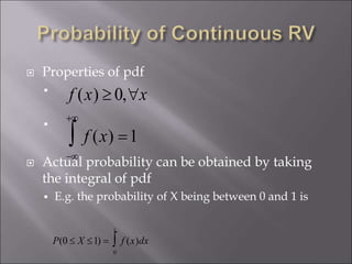
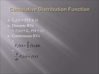
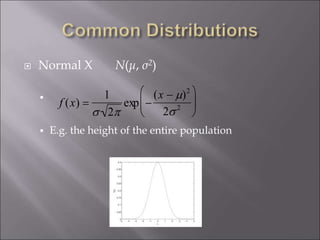
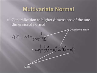
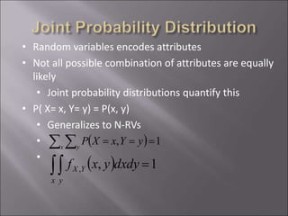
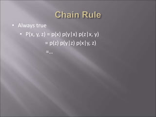
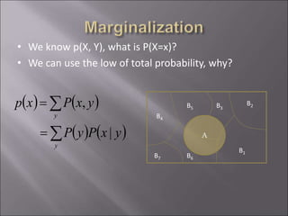
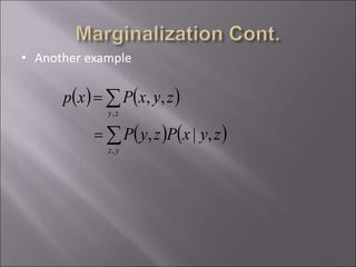
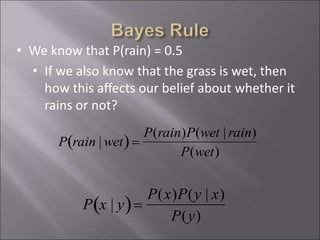
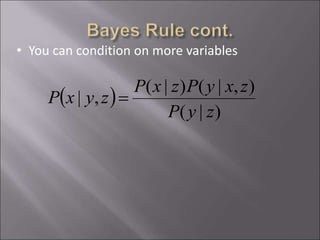
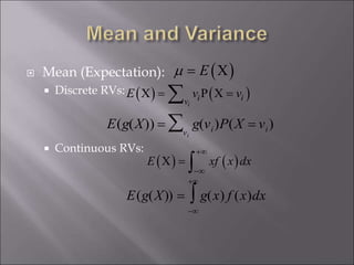
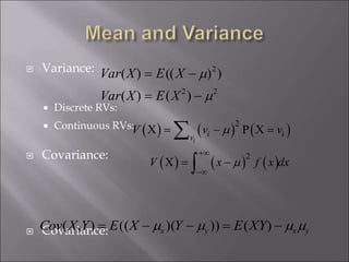
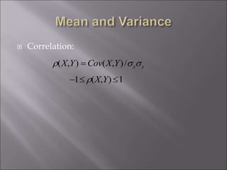
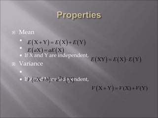
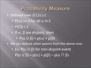
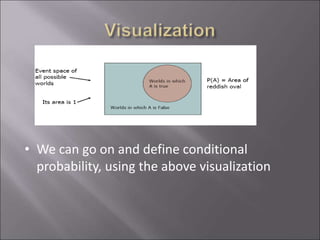
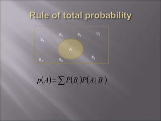
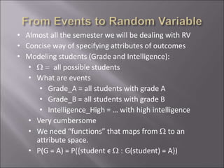
The document provides an overview of probability and statistics, highlighting key concepts such as probability distributions, random variables, and essential statistical principles like conditional probability and independence. It emphasizes the relationship between probability theory and statistical analysis, detailing various probability functions and laws governing random variables. Additionally, the document covers topics like mean, variance, covariance, and the significance of joint and marginal distributions in understanding data relationships.

1. Probability and Statistics:
homework assignment help is most useful online portal for students providing all
type of Online Probability and statistics assignment help Services. These are the
separate articles on probability or the article on statistics. Statistical analysis often
uses probability distributions, and the two topics are often studied together.
However, probability theory contains much that is of mostly mathematical interest
and not directly relevant to statistics. Moreover, many topics in statistics are
independent of probability
theory.
http://www.homeworkassignmenthelp.com/

2. • W : Sample Space, result of an experiment
• If you toss a coin twice W = {HH,HT,TH,TT}
• Event: a subset of W
• First toss is head = {HH,HT}
• S: event space, a set of events:
• Closed under finite union and complements
• Entails other binary operation: union, diff, etc.
• Contains the empty event and W

3. • Defined over (W,S) s.t.
• P(a) >= 0 for all a in S
• P(W) = 1
• If a, b are disjoint, then
• P(a U b) = p(a) + p(b)
• We can deduce other axioms from the above ones
• Ex: P(a U b) for non-disjoint event
P(a U b) = p(a) + p(b) – p(a ∩ b)

4. • We can go on and define conditional
probability, using the above visualization

5. P(F|H) = Fraction of worlds in which H is true that also
have F true
)(
)(
)|(
Hp
HFp
hfp

=

6. A
B1
B2B3
B4
B5
B6B7
 )  )  )= ii BAPBPAp |

7. • Almost all the semester we will be dealing with RV
• Concise way of specifying attributes of outcomes
• Modeling students (Grade and Intelligence):
• W = all possible students
• What are events
• Grade_A = all students with grade A
• Grade_B = all students with grade B
• Intelligence_High = … with high intelligence
• Very cumbersome
• We need “functions” that maps from W to an
attribute space.
• P(G = A) = P({student ϵ W : G(student) = A})

8. W
High
low
A
B A+
I:Intelligence
G:Grade
P(I = high) = P( {all students whose intelligence is high})

9.  Random variables (RVs) which may take on
only a countable number of distinct values
 E.g. the total number of tails X you get if you flip 100
coins
 X is a RV with arity k if it can take on exactly
one value out of {x1, …, xk}
 E.g. the possible values that X can take on are 0, 1, 2,
…, 100

10.  Probability mass function (pmf): P(X = xi)
 Easy facts about pmf
 Σi P(X = xi) = 1
 P(X = xi∩X = xj) = 0 if i ≠ j
 P(X = xi U X = xj) = P(X = xi) + P(X = xj) if i ≠ j
 P(X = x1 U X = x2 U … U X = xk) = 1

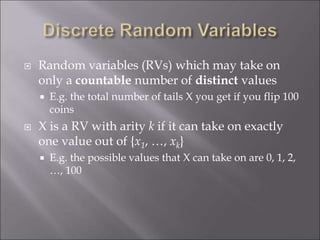
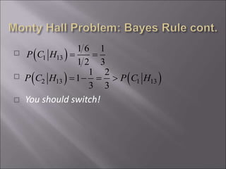
11.  Uniform X U[1, …, N]
 X takes values 1, 2, … N
 P(X = i) = 1/N
 E.g. picking balls of different colors from a box
 Binomial X Bin(n, p)
 X takes values 0, 1, …, n

 E.g. coin flips

p(X = i) =
n
i





pi
(1 p)ni

12.  Probability density function (pdf) instead of
probability mass function (pmf)
 A pdf is any function f(x) that describes the
probability density in terms of the input
variable x.

13.  Properties of pdf


 Actual probability can be obtained by taking
the integral of pdf
 E.g. the probability of X being between 0 and 1 is

f (x)  0,x
f (x) =1



P(0  X 1) = f (x)dx
0
1


14.  FX(v) = P(X ≤ v)
 Discrete RVs
 FX(v) = Σvi P(X = vi)
 Continuous RVs


FX (v) = f (x)dx

v

d
dx
Fx (x) = f (x)

15.  Normal X N(μ, σ2)

 E.g. the height of the entire population

f (x) =
1
 2
exp 
(x  )2
22







16.  Generalization to higher dimensions of the one-
dimensional normal
f r
X
(xi,...,xd ) =
1
(2)d /2

1/2

exp 
1
2
r
x   )
T
1 r
x   )






.
Covariance matrix
Mean

17. • Events and Event spaces
• Random variables
• Joint probability distributions
• Marginalization, conditioning, chain rule,
Bayes Rule, law of total probability, etc.
• Structural properties
• Independence, conditional independence
• Mean and Variance
• The big picture
• Examples

18. • Random variables encodes attributes
• Not all possible combination of attributes are equally
likely
• Joint probability distributions quantify this
• P( X= x, Y= y) = P(x, y)
• Generalizes to N-RVs
•
•
 )  ===x y
yYxXP 1,
 ) =
x y
YX dxdyyxf 1,,

19. • Always true
• P(x, y, z) = p(x) p(y|x) p(z|x, y)
= p(z) p(y|z) p(x|y, z)
=…

20.  )
 )
 )
P X Y
P X Y
P Y
x y
x y
y
=  =
= = =
=
 )
)(
),(
|
yp
yxp
yxP =
But we will always write it this way:
events

21. • We know p(X, Y), what is P(X=x)?
• We can use the low of total probability, why?
 )  )
 )  )

=
=
y
y
yxPyP
yxPxp
|
,
A
B1
B2B3
B4
B5
B6B7

22. • Another example
 )  )
 )  )

=
=
yz
zy
zyxPzyP
zyxPxp
,
,
,|,
,,

23. • We know that P(rain) = 0.5
• If we also know that the grass is wet, then
how this affects our belief about whether it
rains or not?

P rain | wet )=
P(rain)P(wet | rain)
P(wet)
P x | y )=
P(x)P(y | x)
P(y)

24. • You can condition on more variables
 )
)|(
),|()|(
,|
zyP
zxyPzxP
zyxP =

25. • Events and Event spaces
• Random variables
• Joint probability distributions
• Marginalization, conditioning, chain rule,
Bayes Rule, law of total probability, etc.
• Structural properties
• Independence, conditional independence
• Mean and Variance
• The big picture
• Examples

26. • X is independent of Y means that knowing Y
does not change our belief about X.
• P(X|Y=y) = P(X)
• P(X=x, Y=y) = P(X=x) P(Y=y)
• The above should hold for all x, y
• It is symmetric and written as X  Y

27.  X1, …, Xn are independent if and only if
 If X1, …, Xn are independent and identically
distributed we say they are iid (or that they are
a random sample) and we write

P(X1  A1,..., Xn  An ) = P Xi  Ai )
i=1
n

X1, …, Xn ∼ P

28. • RV are rarely independent but we can still
leverage local structural properties like
Conditional Independence.
• X  Y | Z if once Z is observed, knowing the
value of Y does not change our belief about X
• P(rain  sprinkler’s on | cloudy)
• P(rain  sprinkler’s on | wet grass)

29. • P(X=x | Z=z, Y=y) = P(X=x | Z=z)
• P(Y=y | Z=z, X=x) = P(Y=y | Z=z)
• P(X=x, Y=y | Z=z) = P(X=x| Z=z)
P(Y=y| Z=z) We call these factors : very useful concept !!

30. • Events and Event spaces
• Random variables
• Joint probability distributions
• Marginalization, conditioning, chain rule,
Bayes Rule, law of total probability, etc.
• Structural properties
• Independence, conditional independence
• Mean and Variance
• The big picture
• Examples

31.  Mean (Expectation):
 Discrete RVs:
 Continuous RVs:
 )XE =
 )  )X P X
i
i iv
E v v= =
 )  )XE xf x dx


= 

E(g(X)) = g(vi)P(X = vi)vi

E(g(X)) = g(x) f (x)dx




32.  Variance:
 Discrete RVs:
 Continuous RVs:
 Covariance:
 Covariance:
 )  )  )2
X P X
i
i iv
V v v=  =
 )  )  )2
XV x f x dx


= 

Var(X) = E((X  )2
)
Var(X) = E(X2
)  2
Cov(X,Y) = E((X  x )(Y  y )) = E(XY)  xy

33.  Correlation:

(X,Y) = Cov(X,Y)/xy

1 (X,Y) 1

34.  Mean


 If X and Y are independent,
 Variance

 If X and Y are independent,
 )  )  )X Y X YE E E = 
 )  )X XE a aE=
 )  )  )XY X YE E E= 
 )  )2
X XV a b a V =
 )X Y (X) (Y)V V V = 

35.  The conditional expectation of Y given X when
the value of X = x is:
 The Law of Total Expectation or Law of
Iterated Expectation:
 ) dyxypyxXYE )|(*| ==
   === dxxpxXYEXYEEYE X )()|()|()(

36.  The law of Total Variance:

Var(Y) =Var E(Y | X)  E Var(Y | X) 

37. • Events and Event spaces
• Random variables
• Joint probability distributions
• Marginalization, conditioning, chain rule,
Bayes Rule, law of total probability, etc.
• Structural properties
• Independence, conditional independence
• Mean and Variance
• The big picture
• Examples

38. Mode
l
Data
Probability
Estimation/learning

39.  Given observations from a model
 What (conditional) independence assumptions hold?
 Structure learning
 If you know the family of the model (ex,
multinomial), What are the value of the parameters:
MLE, Bayesian estimation.
 Parameter learning

40. • Events and Event spaces
• Random variables
• Joint probability distributions
• Marginalization, conditioning, chain rule,
Bayes Rule, law of total probability, etc.
• Structural properties
• Independence, conditional independence
• Mean and Variance
• The big picture
• Examples

41.  : the car is behind door i, i = 1, 2, 3

 : the host opens door j after you pick door i

iC
ijH
 ) 1 3iP C =
 )
0
0
1 2
1 ,
ij k
i j
j k
P H C
i k
i k j k
=
 =
= 
=
  

42.  WLOG, i=1, j=3


 )
 )  )
 )
13 1 1
1 13
13
P H C P C
P C H
P H
=
 )  )13 1 1
1 1 1
2 3 6
P H C P C =  =

43. 

 )  )  )  )
 )  )  )  )
13 13 1 13 2 13 3
13 1 1 13 2 2
, , ,
1 1
1
6 3
1
2
P H P H C P H C P H C
P H C P C P H C P C
=  
= 
=  
=
 )1 13
1 6 1
1 2 3
P C H = =

44.  )1 13
1 6 1
1 2 3
P C H = =

 You should switch!
 )  )2 13 1 13
1 2
1
3 3
P C H P C H=  = 

45. • P(X) encodes our uncertainty about X
• Some variables are more uncertain that others
• How can we quantify this intuition?
• Entropy: average number of bits required to encode X
P(X) P(Y)
X Y
 )
 )
 )
 )
 ) ==





=
xx
P xPxP
xP
xP
xp
EXH )(log
1
log
1
log

46. • Entropy: average number of bits required to encode X
• We can define conditional entropy similarly
• i.e. once Y is known, we only need H(X,Y) – H(Y) bits
• We can also define chain rule for entropies (not surprising)
 )
 )
 )  )YHYXH
yxp
EYXH PPP =





= ,
|
1
log|
 )  )  )  )YXZHXYHXHZYXH PPPP ,||,, =
 )
 )
 )
 )
 ) ==





=
xx
P xPxP
xP
xP
xp
EXH )(log
1
log
1
log

47. • Remember independence?
• If XY then knowing Y won’t change our belief about X
• Mutual information can help quantify this! (not the only
way though)
• MI:
• “The amount of uncertainty in X which is removed by
knowing Y”
• Symmetric
• I(X;Y) = 0 iff, X and Y are independent!
 )  )  )YXHXHYXI PPP |; =
 





=
y x ypxp
yxp
yxpYXI
)()(
),(
log),();(

48. Republican Democrat Independent Total
Male 200 150 50 400
Female 250 300 50 600
Total 450 450 100 1000
• State the hypotheses
H0: Gender and voting preferences are independent.
Ha: Gender and voting preferences are not independent
• Choose significance level
Say, 0.05

49.  Analyze sample data
• Degrees of freedom =
|g|-1 * |v|-1 = (2-1) * (3-1) = 2
• Expected frequency count =
Eg,v = (ng * nv) / n
Em,r = (400 * 450) / 1000 = 180000/1000 = 180
Em,d= (400 * 450) / 1000 = 180000/1000 = 180
Em,i = (400 * 100) / 1000 = 40000/1000 = 40
Ef,r = (600 * 450) / 1000 = 270000/1000 = 270
Ef,d = (600 * 450) / 1000 = 270000/1000 = 270
Ef,i = (600 * 100) / 1000 = 60000/1000 = 60
Republica
n
Democrat Independen
t
Total
Male 200 150 50 400
Femal
e
250 300 50 600
Total 450 450 100 1000

50.  Chi-square test statistic
 Χ2 = (200 - 180)2/180 + (150 - 180)2/180 + (50 - 40)2/40 +
(250 - 270)2/270 + (300 - 270)2/270 + (50 - 60)2/40
 Χ2 = 400/180 + 900/180 + 100/40 + 400/270 + 900/270 +
100/60
 Χ2 = 2.22 + 5.00 + 2.50 + 1.48 + 3.33 + 1.67 = 16.2







 
= 
vg
vgvg
E
EO
X
,
2
,,2
)(
Republica
n
Democrat Independen
t
Total
Male 200 150 50 400
Femal
e
250 300 50 600
Total 450 450 100 1000

51.  P-value
 Probability of observing a sample statistic as extreme
as the test statistic
 P(X2 ≥ 16.2) = 0.0003
 Since P-value (0.0003) is less than the
significance level (0.05), we cannot accept the
null hypothesis
 There is a relationship between gender and
voting preference

52.  Contact : - 9540660064
 Email : hahassignment@gmail.com
 Visit Us : http://www.homeworkassignmenthelp.com/