Download as PDF, PPTX

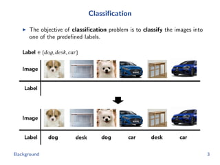
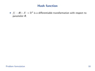
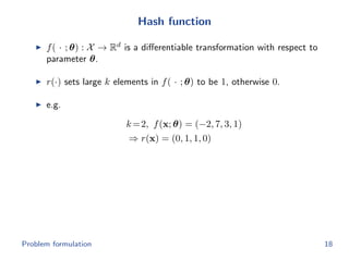
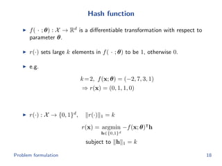
![Triplet loss
(X, y) =
1
T
(a,p,n)∈T
[D2
a,p + α − D2
a,n]+
X : a set of images
y : a set of classes
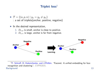
T : a set of triplets(anchor, positive, negative)
α : a margin which is constant
[·]+ = max(·, 0)
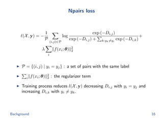
Training process reduces l(X, y) decreasing Da,p and increasing Da,n.
Background 14](https://image.slidesharecdn.com/main-180928092811/85/Efficient-end-to-end-learning-for-quantizable-representations-14-320.jpg)
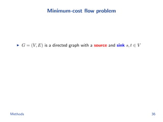
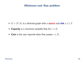
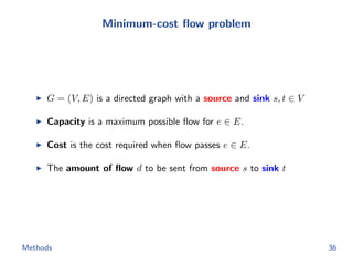
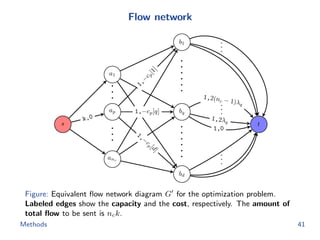
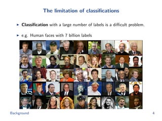
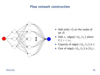
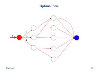
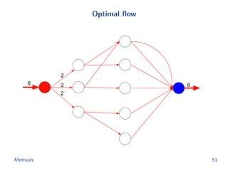
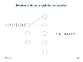
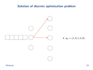
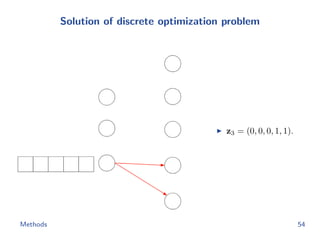
![Flow network construction
c1 = (1, 2, −1, 3, −2)
Capacity of every edge is 1.
Cost of edge(=(ap, bq)) is
−cp[q].
Methods 43](https://image.slidesharecdn.com/main-180928092811/85/Efficient-end-to-end-learning-for-quantizable-representations-52-320.jpg)
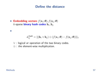
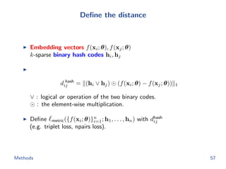
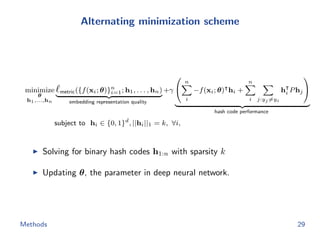
![Metric learning losses
Triplet loss
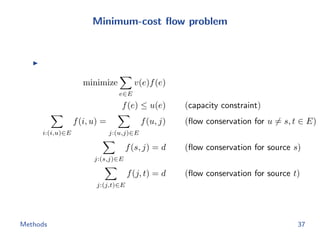
minimize
θ
1
|T |
(i,j,k)∈T
[d hash
ij + α − d hash
ik ]+
triplet(θ; h1,...,n)
subject to ||f(x; θ)||2 = 1
We apply the semi-hard negative mining to construct triplet.
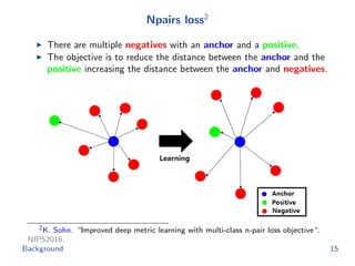
Npairs loss
minimize
θ
−1
|P|
(i,j)∈P
log
exp(−d hash
ij )
exp(−d hash
ij ) + k:yk=yi
exp(−d hash
ik )
npairs(θ; h1,...,n)
+
λ
m i
||f(xi; θ)||2
2
Methods 58](https://image.slidesharecdn.com/main-180928092811/85/Efficient-end-to-end-learning-for-quantizable-representations-69-320.jpg)
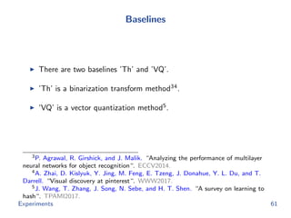
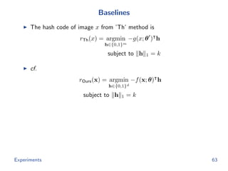
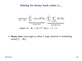
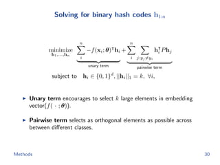
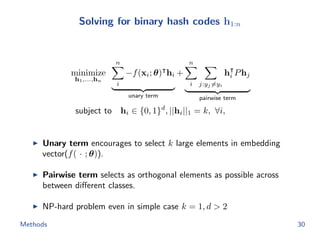
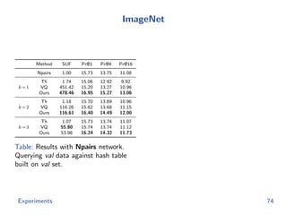
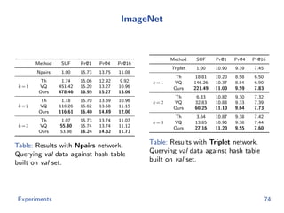
![Baselines
The hash code of image x from ’Th’ method is
rTh(x) = argmin
h∈{0,1}m
−g(x; θ ) h
subject to h 1 = k
cf.
rOurs(x) = argmin
h∈{0,1}d
−f(x; θ) h
subject to h 1 = k
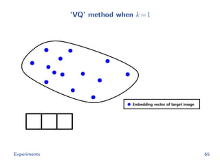
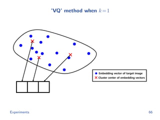
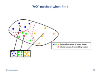
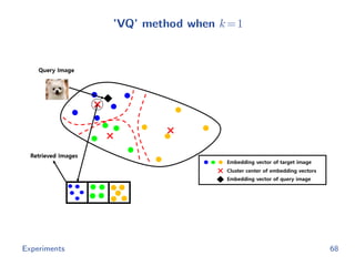
The hash code of image x from ’VQ’ method is
rVQ(x) = argmin
h∈{0,1}d
[ g(x; θ ) − t1 2, · · · , g(x; θ ) − td 2]h
subject to h 1 = k
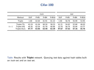
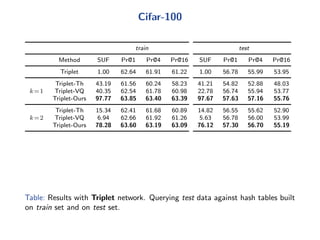
Experiments 63](https://image.slidesharecdn.com/main-180928092811/85/Efficient-end-to-end-learning-for-quantizable-representations-75-320.jpg)

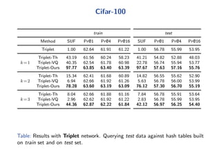
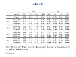
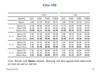
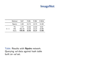

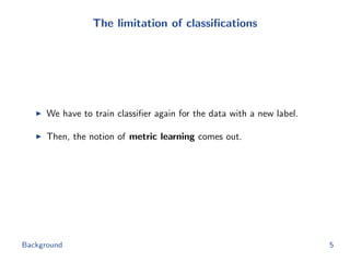
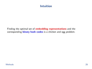
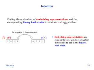
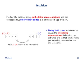
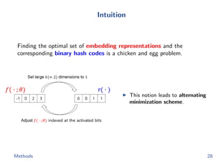
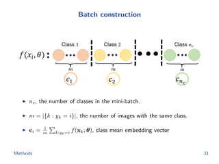
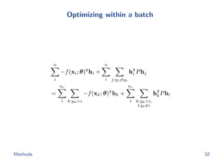
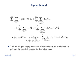
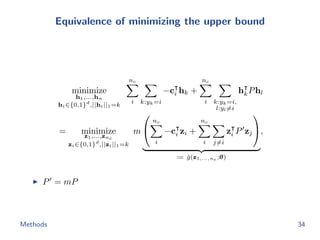
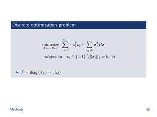
The document discusses efficient end-to-end learning for quantizable representation, focusing on the challenges of image classification with numerous labels and the role of metric learning in addressing these challenges. It presents various methods, including triplet loss and npairs loss, to optimize embedding representations and corresponding binary hash codes, utilizing an alternating minimization framework. The document also outlines experiments comparing proposed methods against baseline approaches to evaluate performance.