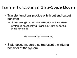
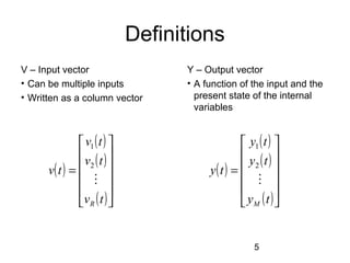
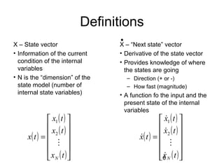
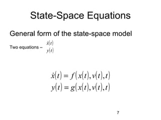
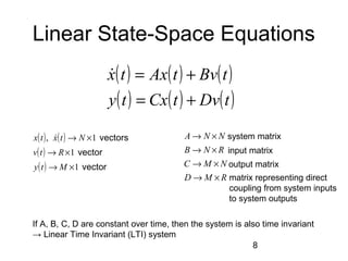
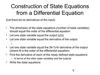
State-space modeling represents systems using matrices and vectors instead of differential/difference equations or transfer functions. It models both the internal state variables and behavior of a system over time. The state-space model defines state, input, output, and next state vectors related by state equations that can be derived from differential equations describing the system. State-space modeling is useful for complex systems as it can handle multiple inputs/outputs and provides insight into the internal workings.

1. State-Space Modeling
David W. Graham
EE 327

2. 2
State-Space Modeling
• Alternative method of modeling a system
than
– Differential / difference equations
– Transfer functions
• Uses matrices and vectors to represent
the system parameters and variables

3. 3
Motivation for State-Space Modeling
• Easier for computers to perform matrix algebra
– e.g. MATLAB does all computations as matrix math
• Handles multiple inputs and outputs
• Provides more information about the system
– Provides knowledge of internal variables (states)
⇒Primarily used in complicated, large-scale
systems

4. 4
Transfer Functions vs. State-Space Models
• Transfer functions provide only input and output
behavior
– No knowledge of the inner workings of the system
– System is essentially a “black box” that performs
some functions
• State-space models also represent the internal
behavior of the system
H(s)X(s) Y(s)

5. 5
Definitions
V – Input vector
• Can be multiple inputs
• Written as a column vector
( )
( )
( )
( )











=
tv
tv
tv
tv
R

2
1
Y – Output vector
• A function of the input and the
present state of the internal
variables
( )
( )
( )
( )











=
ty
ty
ty
ty
M

2
1

6. 6
Definitions
X – State vector
• Information of the current
condition of the internal
variables
• N is the “dimension” of the
state model (number of
internal state variables)
( )
( )
( )
( )











=
tx
tx
tx
tx
N

2
1
X – “Next state” vector
• Derivative of the state vector
• Provides knowledge of where
the states are going
– Direction (+ or -)
– How fast (magnitude)
• A function fo the input and the
present state of the internal
variables
( )
( )
( )
( )











=
tx
tx
tx
tx
N




 2
1

7. 7
State-Space Equations
General form of the state-space model
Two equations –
( )
( )ty
tx
( ) ( ) ( )( )
( ) ( ) ( )( )ttvtxgty
ttvtxftx
,,
,,
=
=

8. 8
Linear State-Space Equations
( ) ( ) ( )
( ) ( ) ( )tDvtCxty
tBvtAxtx
+=
+=
( ) ( )
( )
( ) vector
vector
vectors
1
1
1,
×→
×→
×→
Mty
Rtv
Ntxtx 
RMD
NMC
RNB
NNA
×→
×→
×→
×→ system matrix
input matrix
output matrix
matrix representing direct
coupling from system inputs
to system outputs
If A, B, C, D are constant over time, then the system is also time invariant
→ Linear Time Invariant (LTI) system

9. 9
Construction of State Equations
from a Differential Equation
(Let there be no derivatives of the input)
• The dimension of the state equations (number of state variables)
should equal the order of the differential equation
• Let one state variable equal the output (y(t))
• Let one state variable equal the derivative of the output
• Let one state variable equal the (N-1)-th derivative of the output
(where N is the order of the differential equation)
• Find the derivative of each of the newly defined state equations
– In terms of the other state variables and the outputs
• Write the state equations


10. 9
Construction of State Equations
from a Differential Equation
(Let there be no derivatives of the input)
• The dimension of the state equations (number of state variables)
should equal the order of the differential equation
• Let one state variable equal the output (y(t))
• Let one state variable equal the derivative of the output
• Let one state variable equal the (N-1)-th derivative of the output
(where N is the order of the differential equation)
• Find the derivative of each of the newly defined state equations
– In terms of the other state variables and the outputs
• Write the state equations
