Stability and stabilization of discrete-time systems with time-delay via Lyapunov-Krasovskii functional

Bemri H’mida et al. Int. Journal of Engineering Research and Applications www.ijera.com
ISSN: 2248-9622, Vol. 5, Issue 11, (Part - 2) November 2015, pp.40-46
www.ijera.com 40 | P a g e
Stability and stabilization of discrete-time systems with time-delay
via Lyapunov-Krasovskii functional
Bemri H’mida1
, Mezlini Sahbi2
and Soudani Dhaou3
Tunis El Manar University
Laboratory of Research on Automatic (LARA)
National Engineers School of Tunis
BP 37, Belvedere 1002 Tunis. Tunisia.
ABSTRACT
The stability and stabilization problems for discrete systems with time-delay are discussed .The stability and
stabilization criterion are expressed in the form of linear matrix inequalities (LMI). An effective method
allowing us transforming a bilinear matrix Inequality (BMI) to a linear matrix Inequality (LMI) is developed.
Based on these conditions, a state feedback controller with gain is designed. An illustrative numerical example
is provided to show the effectiveness of the proposed method and the reliability of the results.
Keywords - Asymptotic stability; discrete-time systems; Lyapunov functional; Lyapunov-Krasovskii method;
linear matrix inequalities (LMI); time-delay.
I. INTRODUCTION
Time delay is an important factor that may affect
the performance of dynamical systems. It can even,
in same situation, cause instability of a system that
we would like to control if the presence of such time-
delay during the design phases is not taken into
account .For linear systems with time delay; we have
seen an increasing interest during the last two
decades. There are numerous results in the literature
on time-delay systems [4,7,8,17].However; most
results are focused on the continuous-time linear
systems with time delay. Stability, stabilization and
control problems for this system have been studied
and numerous results are available in the literature
such as [3,5,9]. However, for discrete-time linear
systems with time-delay only few results have been
reported in the literature. We believe that the main
reason for this is that these systems can be
transformed to equivalent systems without time-delay
and then current results on stability, stabilization and
control design can be applied.
Time delay is frequently encountered in many
fields of engineering systems, such as manufacturing
system, telecommunication, economic system, and
chemical engineering system. It is generally regarded
as a main source of stability and poor performance
[12,14,19]. Therefore, the problems of stability
analysis and stabilization of time-delay systems are
important both in theory and practice, and are thus of
interest to many researchers. Commonly, the
approaches for solving time-delay systems can be
classified into two types. Delay-dependent conditions
[1,2,13], which include information on the size of
delays, and delay-independent conditions, which are
applicable to delays of arbitrary size. Since the
stability of a system depends explicitly on the time-
delay, a delay-independent condition is more
conservative, especially for small delays, while a
delay-dependent condition is usually less
conservative.
Due to the development in the field of
microelectronics analog controllers are yielding their
places to digital computers. Indeed, and giving the
importance of these control systems, we are using
methods and numerical models to analyze and / or to
control industrial processes.
Two types of representation are available to
model a continuous or discrete dynamic system
namely the external representation that uses input-
output relations (transfer function) or the internal
representation (matrix) of dynamic system which is
based on the concept of state. To implement such a
control structure and ensure the desired objectives, a
modeling in the generally required discrete-time
analog systems is needed.
Digital control of physical systems requires,
usually the development of discrete models. Several
modeling strategies, developed in the literature
reflecting a meaningful description of dynamical
systems to be studied led to mathematical tools
leading generally to linear or non-linear models with
or without delays whose behavior may be more or
less close to the real system [10,11,15,18]. These
models are described by relations between input
variables and output variables that can be modified
by inputs considered as secondary (disturbances) that
always exist in practice.
The initial modeling of a discrete time-delays
system often leads to writing a recurrent equation
between different terms of the input and output
RESEARCH ARTICLE OPEN ACCESS

sequences. This formulation of the recurrent equation
is well suited for numerical calculation. This is the
form in which these algorithms are digital control
methods. The system is fully defined and the
recurrent equation can be solved if the initial
conditions are specified.
The analysis of the stability of delays systems
has been conducted in the literature by numerous
fundamental researches that depend on the type of
systems considered and the scope. There are many
study methods of the stability of linear discrete time-
delay systems. These stability criteria can be
classified into two main categories namely the
frequency criterion using the notion of the
characteristic equations and the time criterion based
on Lyapunov theory.
This paper is organized as follows. In Section 2,
the problem is stated and the objective of the paper is
formulated. The problems of stability for the given
system is examined and delay-dependent or
independent sufficient condition is developed in
section 3.We continue in section 4, to investigate the
problem of stability and establish delay-dependent
conditions. In addition, a design algorithm that
stabilizes the resulting closed-loop system is
provided. A numerical example is given in section 5
to illustrate the proposed theoretical results.
II. FORMULATION OF THE PROBLEM AND
SOME PRELIMINARY
R Real vector space.
*
( ) n n
ij
F f R  Real matrix.
T
F Transpose of the matrix F.
> 0F Positive definite matrix.
0F  Positive semi-definite matrix.
( )F Eigenvalue of the matrix F.
( ) || F ||F  Singular value of the matrix.
max
| F || ( )| T
F F Euclidean norm of the matrix F.
Considering the dynamics of the discrete system
with time-delays defined by the following equation:
0 1( 1) ( ) ( ) ( )    x k A x k A x k q Bu k (1)
Where ( ) n
x k R is the state at time k .
 x( ) ( ), , 1,..,0q q        represents the initial
condition.
*n n
i
A R are constant matrices of appropriate size.
1,2,.....q  is a positive integer representing the time
delay existing in the system.
Whether V :
n
R R in such a way that ( )V x is
bounded for all x is bounded.
The aim of this paper is to establish sufficient
conditions that guarantee the stability of the class of
system (1). Based on stability conditions, the
stabilization problem of this system (1) will be
handled, too. The control law is given with a memory
less state-feedback as: 1 2
( ) ( ) , ( )u k L x k L L L  
Where L is the control gain to be computed.
III. STABILITY ANALYSIS
The stability of discrete time-delay systems has
received much attention in the past several years [6,
7]. In the literature, there are some necessary and
sufficient stability conditions for these systems.
Based on these results, some necessary and sufficient
stability conditions for discrete-time delay systems
can be obtained. Roughly speaking, the stability of a
system is its ability to resist any unknown small
influences. Since in reality disturbances are always
encountered, stability is an important property of any
control system, delayed or non delayed.
In this section, LMIs-based conditions of delay-
dependent or independent stability analysis will be
considered for discrete-time systems with time-
delays. The following result gives sufficient
conditions to guarantee that the system (1) for
( ) 0 , 0u k k  is stable.
Fact 1: for any positive scalar α and for any two
vectors x and y, we present the following inequality:
1T T T T
x y y x x x y y 
  
(2)
Note that:
 : || || <n
V x R x  
(3)
Lemma 1: [16] the zero solution of the difference
system is asymptotically stable if there exists a
positive definite ( ( )) : n
V x k R R
 knowing that there
is a > 0 as:
2
( ( )) ( ( 1)) ( ( )) || ( ) ||V x k V x k V x k x k      (4)
The above inequality is true throughout the linear
resolution of the discrete system. If the above
condition is valid for all ( )x k V , the zero solution
of the difference system is locally asymptotically
stable.
Lemma 2: [16] for any constant symmetric matrix:
*
, > 0
n n T
M R M M  ,  scalar as  / 0Z 
 , and
the vector function  : 0,
n
W R  , we have the
following inequality:
 
1 1 1
0 0 0
(i) (i) (i) (i)
T
T
i i i
w M w w M w
  

  
  
    
   
   
   
   (5)
A-Delay-dependent stability:
This group includes exact algebraic stability
criteria depending on the delay and on the system

constants and stability criteria which yield an upper
bound of the admissible delay.
Using the stated theorem in the following and
previously stated lemmas we can determine the
asymptotic stability of the linear discrete system that
is presented in equation (1).
Theorem 1:
The discrete time-delay system (1) is
asymptotically stable for any delay > 0q , if there
exist symmetric positive definite
matrix > 0
T
P P , > 0
T
G G and > 0
T
W W
satisfying the following matrix inequalities:
1
(1,1) 0 0
0 (2,2) 0 0
0 0 (3,3)
  
 
 
 
 
 
(6)
Such as:
2
0 0 0 0
(1,1) A PA A P A G W P
T T
q     (7)
1
1 1 1 1
(2,2) P W
T T
A A A A
   (8)
(3,3) Gq  (9)
Evidence: Consider the Lyapunov function defined as
follows:
1 2 3
( ( )) ( ( )) ( ( )) ( ( ))V y k V y k V y k V y k   (10)
Where:
1
( ( )) ( ) ( )
T
V y k x k P x k   (11)
 
1
2
( ( )) (i) (i)
k
T
i k q
V y k q k i x G x

 
      (12)
1
3
( ( )) (i) (i)
k
T
i k q
V y k x W x

 
   (13)
 ( ) ( ), ( )y k x k x k q  (14)
With > 0
T
P P , > 0
T
G G and > 0
T
W W is
symmetric positive definite solutions of (6)
and  ( ) ( ), ( )y k x k x k q  .
Then the difference of ( ( ))V y k along the path of the
solution (4) is given by:
1 2 3
( ( )) ( ( )) ( ( )) ( ( ))V y k V y k V y k V y k       (15)
With:
   
1 1 1
0 1 0 1
0 0 0 1
1 0 1 1
( ( )) ( ( 1)) ( ( ))
( ) ( ) ( ) ( ) ( ) ( )
( ) ( ) ( ) ( )
( ) ( ) ( ) ( )
T T
T T T T
T T T T
V y k V x k V x k
A x k A x k q P A x k A x k q x k Px k
x k A PA P x k x k A PA x k q
x k q A PA x k x k q A PA x k q
   
     
    
    
  
(16)
 
2 2 2
1
1
( ( )) ( ( 1)) ( ( ))
( ) ( )
( ) ( ) ( ) ( )
k
T
i k q
k
T T
i k q
V y k V x k V x k
q k i x i Gx i
qx k Gx k x i Gx i

 

 
   
   
 
 
 
 


(17)
3 3 3
1
( ( )) ( ( 1)) ( ( ))
( ) W ( )
( ) W ( ) ( ) W ( )
k
T
i k q
T T
V y k V x k V x k
x i x i
x k x k x k q x k q

 
   
 
   
 
 
 
 (18)
Applying the Fact 1 in equation (16), the following
inequality is obtained:
0 1 1 0
0 0 1 1
2 1
( ) ( ) ( ) ( )
( ) ( ) ( ) ( )
T T T T
T T T T
x k A PAx k q x k q A PA x k
x k A P A x k x k q A Ax k q 
  
  
 (19)
Therefore:
2
1 0 0 0 0
1
1 1 1 1
( ( )) ( ) ( )
( ) ( )
T T T
T T T
V y k x k A PA A P A P x k
x k q A PA A A x k q


    
   
  
  
(20)
Thus the expression (15) of ( ( ))V y k is rewritten as
follows:
0 0 0 0
1 1 1 1
2
1
1
( ( )) ( ) ( )
( ) ( ) ( ) ( )
( ) ( ) ( )W ( ) ( )W ( )
T T T
T T T T
k
T T T
i k q
x k q A PA A A x k q qx k Gx k
x i Gx i x k x k x k q x k q



 
    
     
    
  
  

(21)
Which is equivalent to
0 0 0 0
1 1 1 1
2
1
1
( ( )) ( ) ( )
( ) ( )
( ) ( )
T T T
T T T
k
T
i k q
V y k x k A PA A P A qG W P x k
x k q A PA A A W x k q
x i Gx i



 
      
     

  
  

(22)
By using Lemma 2, we obtain the following
inequality:
1 1 1
1 1
( ) ( ) ( ) ( )
T
k k k
T
i k q i k q i k q
x i qG x i x i Gx i
q q
  
     

   
   
   
   (23)
It follows that:
2
0 0 0 0
1
1 1 1 1
1
( ( )) ( ) ( )
( ) ( )
( ) ( ) ( ) ( )
( ) W ( ) ( ) W ( )
T T T
T T T
k
T T
i k q
T T
x k q A PA A A x k q
qx k Gx k x i Gx i
x k x k x k q x k q



 
   
    
  
   
  
  


(24)
From Fact 1 we get the following expression:

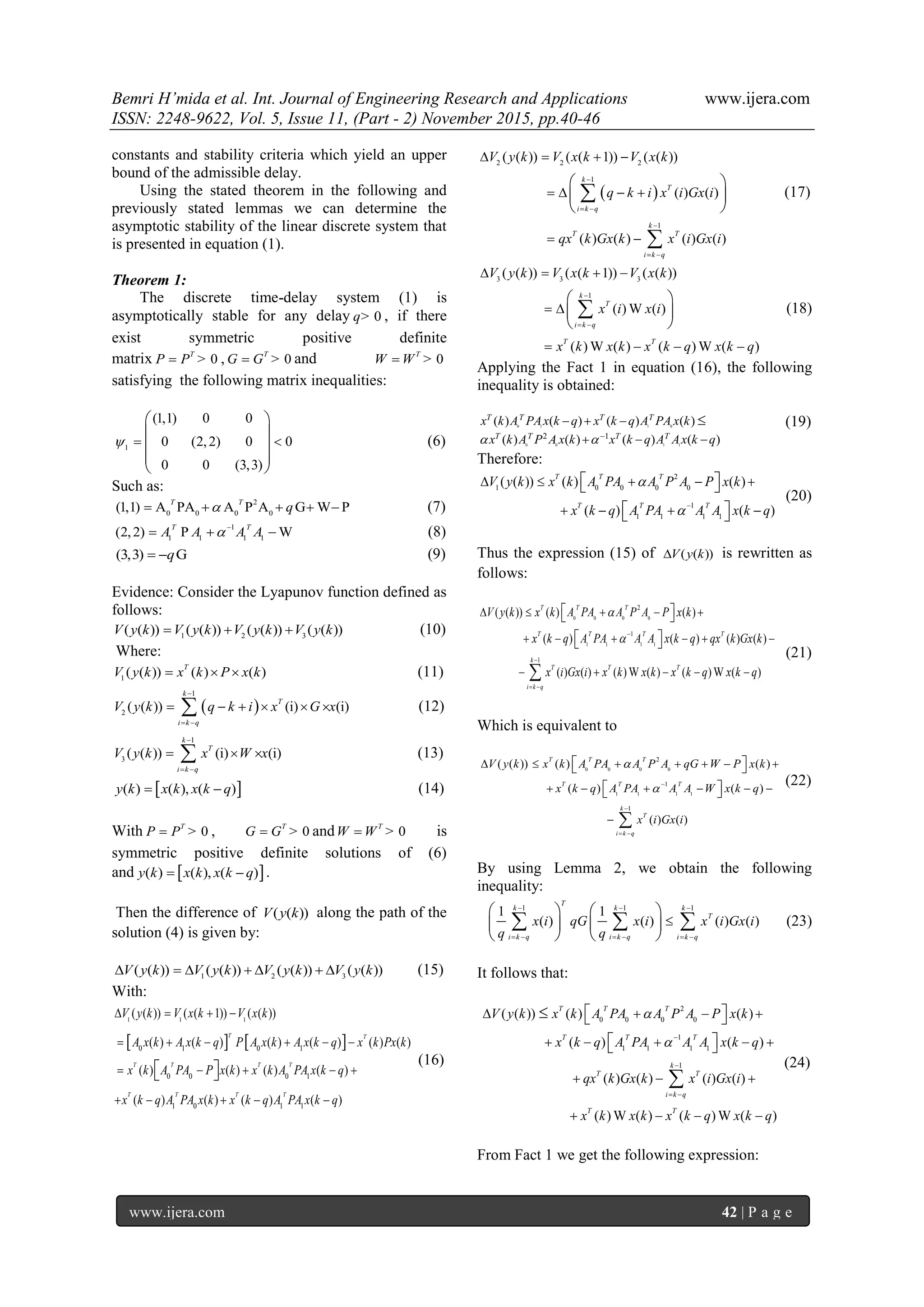
0 0 0 0
1 1 1 1
2
1
1
( ( )) ( ) ( )
( ) ( )
( ) ( )
T T T
T T T
k
T
i k q
A A
V y k x k A PA A P A qG W P x k
x k q PA A W x k q
x i Gx i



 
       
       



(25)
Using Lemma 2, equation (25) will be rewritten as
follows:
2
1
1 1
0 0 0 0
1 1 1 1
( ) ( )
( ( )) ( ) ( )
1 1
( ) ( )


 
   
    
      

 
 
   
 
   
 
    
        
 
 
T T T
T T T
T
k k
i k q i k q
x k A PA A P A qG W P x k
V y k x k q A PA A A W x k q
x i qG x i
q q
(26)
2
1
1 1
1 1 1 1
1
( ) ( )
( ) ( )
1 1
( ) ( )
1
( ), ( ), ( )
(1,1) 0 0
0 (2, 2) 0
0 0 (3,3)
T T T
T T T
T
k k
i k q i k q
o o o o
T
k
T T
i k q
x k A PA A P A qG W P x k
x k q A PA A A W x k q
x i qG x i
q q
x k x k q x i
q
x



 
   

 
    
     

 
 
  
  
   
   
   
  
     
 
 
 
 
 
 

 

1
0
( )
( )
1
( )
( ) ( )
k
i k q
T
k
x k q
x i
q
y k y k

 

 
 
 
 
 
  
  
  
  

(27)
With:
1
( )
( ) ( )
1
( )
k
i k q
x k
y k x k q
x i
q

 
 
 
 
 
 
 
  
  
  

(28)
Where:
0
( ( )) ( ) ( )T
V y k y k y k    (29)
Thus the condition (6) is satisfied, then
( ( ))V y k 0,
 x(k) 0 which allowed us to conclude that the
system defined in equation (5) is asymptotically
stable.
Finally we conclude that ( ( ))v y k is negative
definite; namely, there is a number    such that
2
( ( )) ( )v y k y k   and, consequently, the asymptotic
stability of the system follows immediately from
Lemma 1.
B- Delay-independent stability:
Delay-independent stability criteria are very
useful, since in reality it is difficult to estimate the
delays, especially if those delays are time-varying
and/or state-dependent.
Theorem 2:
asymptotically stable, if there exist symmetric
positive definite matrix > 0
T
N N and
> 0
T
S S such that following linear matrix
inequality (LMI) hold:
0
2 1
0 1
0
0
0
T
T
T T
N S A S
N A S
A S A S S





 
 
 
 
 
. (30)
Proof. Let the Lyapunov functional be:
1
( ( )) ( )Sx( ) ( ) ( )
q
T T
j
V x k x k k x k j Nx k j

    (31)
> 0
T
N N and > 0
T
S S .
The forward difference along the solutions of system
(1) is:
   0 1 0 1
0 0 0 1
0 1 1 1
( ) ( )
( ) ( )
( ( )) ( ) ( ) ( ) ( )
( )S ( ) ( )N ( )
( ) ( )
T
T
T T T
T T
T T
x k x k
A SA S N A SAx k x k
A SA A SA N
V y k A x k A x k q S A x k A x k q
x k x k N x k q x k q
x k q x k q

 
 

    
  
    
          

(32)
If the following equation is satisfied:
0 0 0 1
0 1 1 1
0
T T
T T
A SA S N A SA
A SA A SA N
  
 
  
 (33)
Then
 
0 0 0 0 0 10 1
0 1 0 1 1 11 1
0
0 1
1
0
0
0
0
0
  
 



 
    
    
    
  
  
   
T T TT
T T TT
T
T
A SA S N A SA A SAA SA N S
NA SA A SA A SAA SA N
N S
N
A
S A A
A
(34)
Using Schur complement [5], it is easy to see that the
condition (34) is equivalent to:
0
1
1
0 1
0
0 0
T
T
T T
N S A S
N A S
A S A S S




 
 
 
 
 
(35)
Note that the condition (35) is not LMI condition
due to the existence of the term 1
S
 . Pre and post
multiply (36) with dig {I, I, S } we obtain LMI
condition (31).
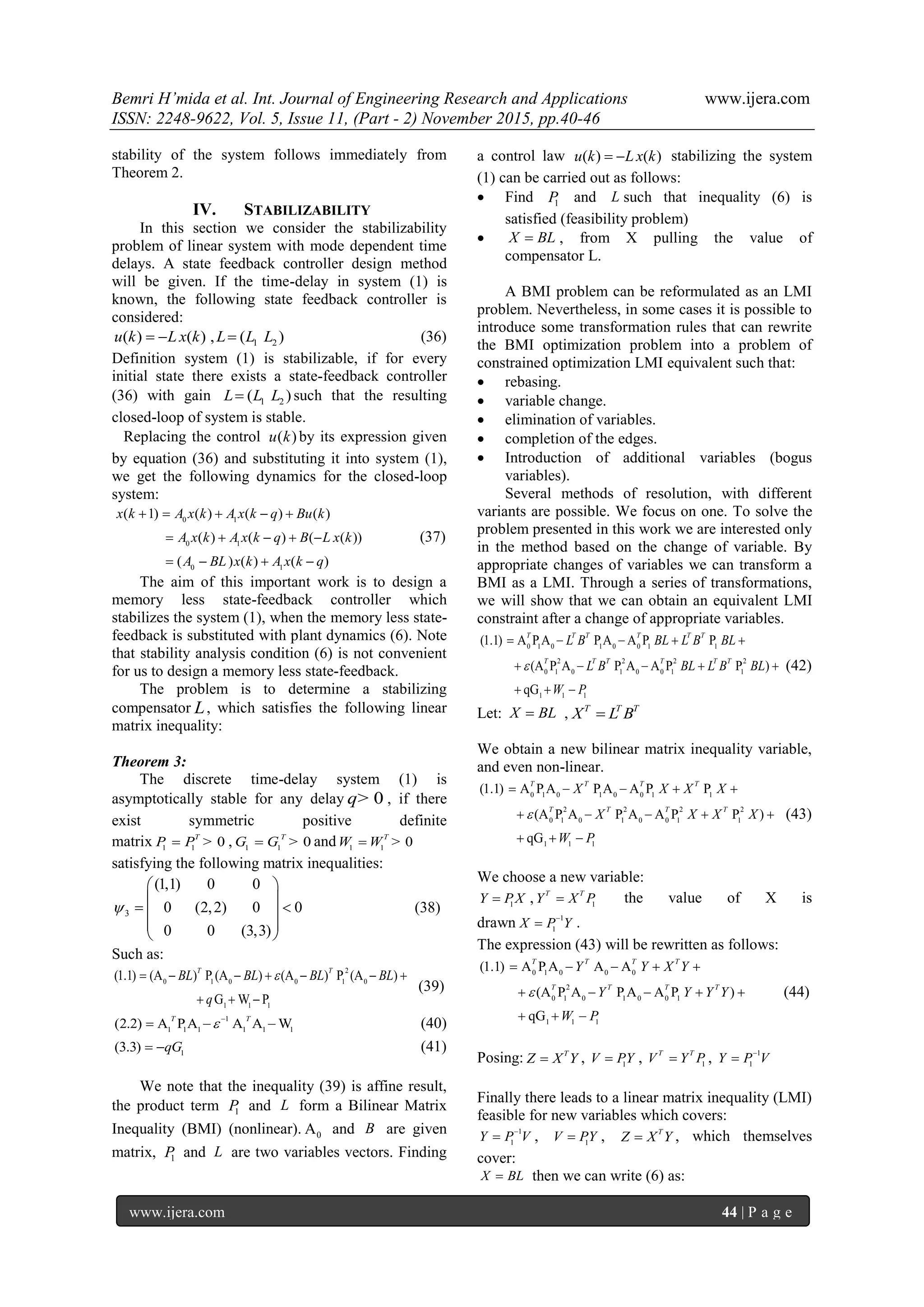
Thus the condition (31) is satisfied, then
(y( ))V k 0,
 ( ) 0x k  Which allowed us to conclude that the
system defined in equation (5) is asymptotically
stable.
Finally we conclude that (y( ))v k is negative
definite; namely, there is a number    such that
2
(y( )) ( )v k y k   and, consequently, the asymptotic

stability of the system follows immediately from
Theorem 2.
IV. STABILIZABILITY
In this section we consider the stabilizability
problem of linear system with mode dependent time
delays. A state feedback controller design method
will be given. If the time-delay in system (1) is
known, the following state feedback controller is
considered:
1 2( ) ( ) , ( )u k L x k L L L   (36)
Definition system (1) is stabilizable, if for every
initial state there exists a state-feedback controller
(36) with gain 1 2( )L L L such that the resulting
closed-loop of system is stable.
Replacing the control ( )u k by its expression given
by equation (36) and substituting it into system (1),
we get the following dynamics for the closed-loop
system:
0 1
0 1
0 1
( 1) ( ) ( ) ( )
( ) ( ) ( ( ))
( ) ( ) ( )
x k A x k A x k q Bu k
A x k A x k q B L x k
A BL x k A x k q
    
    
   
(37)
The aim of this important work is to design a
memory less state-feedback controller which
stabilizes the system (1), when the memory less state-
feedback is substituted with plant dynamics (6). Note
that stability analysis condition (6) is not convenient
for us to design a memory less state-feedback.
The problem is to determine a stabilizing
compensator L, which satisfies the following linear
matrix inequality:
Theorem 3:
asymptotically stable for any delay > 0q , if there
exist symmetric positive definite
matrix 1 1
> 0
T
P P , 1 1
> 0
T
G G and 1 1
> 0
T
W W
satisfying the following matrix inequalities:
3
(1,1) 0 0
0 (2,2) 0 0
0 0 (3,3)

 
 
  
 
 
(38)
Such as:
2
0 1 0 0 1 0
1 1 1
(1.1) (A ) P (A ) (A ) P (A )
G W P
T T
BL BL BL BL
q
      
  
(39)
1
1 1 1 1 1 1
(2.2) A PA A A W
T T

   (40)
1
(3.3) qG  (41)
We note that the inequality (39) is affine result,
the product term 1P and L form a Bilinear Matrix
Inequality (BMI) (nonlinear). 0A and B are given
matrix, 1P and L are two variables vectors. Finding
a control law ( ) ( )u k L x k  stabilizing the system
(1) can be carried out as follows:
 Find 1P and L such that inequality (6) is
satisfied (feasibility problem)
 X BL , from X pulling the value of
compensator L.
A BMI problem can be reformulated as an LMI
problem. Nevertheless, in some cases it is possible to
introduce some transformation rules that can rewrite
the BMI optimization problem into a problem of
constrained optimization LMI equivalent such that:
 rebasing.
 variable change.
 elimination of variables.
 completion of the edges.
 Introduction of additional variables (bogus
variables).
Several methods of resolution, with different
variants are possible. We focus on one. To solve the
problem presented in this work we are interested only
in the method based on the change of variable. By
appropriate changes of variables we can transform a
BMI as a LMI. Through a series of transformations,
we will show that we can obtain an equivalent LMI
constraint after a change of appropriate variables.
0 1 0 1 0 0 1 1
2 2 2 2
0 1 0 1 0 0 1 1
1 1 1
(1.1) A PA PA A P P
(A P A P A A P P )
qG
T T T T T T
T T T T T T
L B BL L B BL
L B BL L B BL
W P

    
    
  
(42)
Let: X BL , T T T
X L B
We obtain a new bilinear matrix inequality variable,
and even non-linear.
0 1 0 1 0 0 1 1
2 2 2 2
0 1 0 1 0 0 1 1
1 1 1
(1.1) A P A P A A P P
(A P A P A A P P )
qG
T T T T
T T T T
X X X X
X X X X
W P

    
    
  
(43)
We choose a new variable:
1
Y PX , 1
T T
Y X P the value of X is
drawn 1
1
X P Y

 .
The expression (43) will be rewritten as follows:
0 1 0 0 0
2
0 1 0 1 0 0 1
1 1 1
(1.1) A P A A A
(A P A P A A P )
qG
T T T T
T T T T
Y Y X Y
Y Y Y Y
W P

    
    
  
(44)
Posing: T
Z X Y , 1
V PY , 1
T T
V Y P , 1
1
Y P V


Finally there leads to a linear matrix inequality (LMI)
feasible for new variables which covers:
1
1
Y P V

 , 1
V PY , T
Z X Y , which themselves
cover:
X BL then we can write (6) as:

0 1 0 0 0
2
0 1 0 0 0
1 1 1
(1.1) A P A A A
(A P A A A )
qG
T T T
T T T T
Y Y Z
V V Y Y
W P

    
    
  
(45)
1
1 1 1 1 1 1
(2.2) P W
T T
A A A A
   (46)
1
(3.3) Gq  (47)
From V is pulled Y, from Y is pulled X then pulls the
expression of L.
V. NUMERICAL EXAMPLE
To illustrate the usefulness of the previous
theoretical results, let us give the following numerical
examples.
Consider the linear discrete time delay system
autonomous defined by the following equation:
0.1 0.02 0.1 0.01 0
( 1) ( ) ( 1) ( )
0.1 0.15 0.2 0.2 1
x k x k x k u k    

     
     
     
(37)
with:
0
0.1 0.02
0.1 0.15
A 

 
 
 
, 1
0.1 0.01
0.2 0.2
A 
 
 
 
and
0
1
B 
 
 
 
A-Applying Theorem 1 to the equation defined in
system (1) and through the relationship (6) .Matrix P,
W and G symmetric positive definite which satisfy
the sufficient condition for stability is obtained:
3.2162 0.0172
0.0172 3.1592
P 
 
 
 
,
1.0696 0.0055
0.0055 1.0555
G



 
 
 
and
1.1628 0.0712
0.0712 1.1295
W 
 
 
 
B-Applying Theorem 2 to the equation defined in
system (1) and through the relationship (30).Matrix N
and S symmetric positive definite which satisfy the
sufficient condition for stability is obtained:
0.1158 1.2007
1.2007 1.0573
N 
 
 
 
and
0.6163 1.6801
1.6801 1.0583
S 
 
 
 
C-Let us now, see how we can use the design
algorithm of theorem3, to determinate the controller
gain  1 2
,L L L . For this purpose let us consider the
following data:
0
0.1 0.02
0.1 0.15
A 

 
 
 
, 1
0.1 0.01
0.2 0.2
A 
 
 
 
and
0
1
B 
 
 
 
Using this data, solving LMIs (38) gives the
following feasible solution:
1
3.2162 0.0172
0.0172 3.1592
P 
 
 
 
, 1
1.0696 0.0055
0.0055 1.0555
G



 
 
 
, 1
1.1628 0.0712
0.0712 1.1295
W 
 
 
 
0.1465 -0.0072
13.6978 -0.6734
V  
 
 
 
1
1Y P V

0.0228 -0.0011
4.2589 -0.2094
Y  
 
 
 
1
1X P Y

0 0
1.3242 -0.0651
X  
 
 
 
X BL
Which gives the following gain:
 1.3242 0.0651L  
VI. CONCLUSION
In this paper we have investigated the stability
and stabilization of discrete time systems with time-
delay. Moreover, we have got same equivalent
stability conditions which are presented as LMI and
thus easy to test, using the Lyapunov function
approach .Furthermore; we have designed a feedback
controller with gain based on one of these stability
conditions. Finally, we have used a numerical
example illustrating effectiveness of the proposed
method.
REFERENCES
[1] H. Gao, J. Lam, C. Wang, Y. Wang. Delay-
dependent output-feedback stabilization of
discrete-time systems with time-varying state
delay. IEE Proceedings -Control Theory and
Applications, vol. 151, no. 6, pp. 691-698,
2004.
[2] K. Ramakrishnan, G. Ray. Delay-range-
dependent stability criterion for interval
time-delay systems with nonlinear
perturbations. International Journal of
Automation and Computing, vol. 8, no. 1,
pp. 141-146, 2011.
[3] Li,X. and de Souza,C.E. Delay-dependent
robust stabiliy and stabilization of uncertian
linear delay systems: a linear matrix
inquality approach. IEEE Trans, Automat.
Control,42(8),pp1144-1148), 1997.
[4] Malek-Zavarei,M. and Jamshichi,M.:Time-
delay systems analysis and applications.
North-Holland, system control series.1987.
[5] Boyd, L. El Ghaoui, E. Feron and V.
Balakrishnan: Linear Matrix Inequalities in
Systems and Control Theory, SIAM,
Philadelphia , PA, 1994.
[6] H. Lin and P.J. Antsaklis, Stability and
stabilizability of switched linear systems: a
survey of recent results, IEEE Transactions

on Automatic Control, vol. 54, pp. 308–322,
2008.
[7] Sreten B. Stojanović, Dragutin Lj.
Debeljković, Ilija Mladenović: A Lyapunov-
Krasovskii Methodology for Asymptotic
Stability of discrete Time Delay Systems.
Serbian Journal Of Electrical Engineering
vol. 4, n°. 2 , pp109-117, Nov 2007.
[8] S. B. Stojanovic and D. Lj. Debeljkovic : On
the Asymptotic Stability of Linear Discrete
Time Delay Autonomous Systems: New
Results.International Journal of Information
and Systems Sciences Computing and
Information vol 1, n° 3-4, pp 413-419, 2012.
[9] K. Ratchagit and V. N. Phat: Stability
Criterion for Discrete-Time Systems.
Hindawi Publishing Corporation,Journal of
Inequalities and Applications , ID 201459, 6
doi:10.1155/2010/201459,2010.
[10] V.L. Kharitonov, A.P. Zhabko: Lyapunov–
Krasovskii Approach to the Robust Stability
Analysis of Time-Delay Systems, Automatica
39, pp. 15-20, 2003.
[11] M. Fu, H. Li, S.I. Niculescu: Robust
Stability and Stabilization of Time-Delay
Systems via Integral Quadratic Constraint
Approach, Stability and Control of Time-
delay Systems(L. Dugard and E. Verriest,
Eds.), Springer-Verlag, London, pp. 101-
116, 1998.
[12] J. Chen, Latchman H.A.: Asymptotic
Stability Independent of Delays: Simple
Necessary and Sufficient Conditions,
Proceedings of American Control
Conference, Baltimore, USA, pp. 1027-
1031, 1994.
[13] J.H. Kim, E.T. Jeung, H. B. Park: Robust
Control for Parameter Uncertain Delay
Systems in State and Control Input,
Automatica 32(9) , pp.1337-1339 1996.
[14] T. Mori: Criteria for Asymptotic Stability of
Linear Time Delay Systems, IEEE
Trans.Autom. Control, Vol. 30, pp. 158-160,
1985.
[15] K. Gu, V. Kharitonov, J. Chen: Stability of
Time-Delay Systems (Control Engineering),
Berlin, Springer, 2003.
[16] R. P. Agarwal: Difference Equations and
Inequalities: Theory, Methods and
Applications, vol. 155 of Monographs and
Textbooks in Pure and Applied
Mathematics, Marcel Dekker, New York,
NY, USA, 1992.
[17] B. H’mida, M. Sahbi, S. Dhaou: Stability of
a linear discrete system with time delay via
Lyapunov-Krasovskii functional.
International Journal of Scientific Research
& Engineering Technology (IJSET). ISSN:
2356-5608, Vol.3, issue 3, Copyright IPCO-
pp.62-67, 2015.
[18] B. H’mida, M. Sahbi, S. Dhaou: Discrete-
Time Approximation of Multivariable
Continuous-Time Delay Systems, IGI
Global: Handbook of Research on Advanced
Intelligent Control Engineering and
Automation, pp516-542, DOI: 10.4018/978-
1-4666-7248-2.ch019, January-2015.
[19] B. H’mida, M. Sahbi, S. Dhaou:
Discretizing of linear systems with time-
delay Using method of Euler's and Tustin's
approximations, International Journal of
Engineering Research and Applications
(IJERA), ISSN: 2248-9622, Vol. 5 -Issue 3,
March-2015.
Authors’ information
Bemri H'mida was born in Tunisia. He
received the scientific degree in mathematics,
physics and computer science within the
Faculty of Sciences of Tunis (FST) in
2003.He received the degree of MA within the
Faculty of Sciences of Tunis (FST) in
2005.He received the certificate of Aptitude Teaching of Second
Degree (CAPES) in 2008.He has been working as a teacher in 2
Mars1934 secondary school in Siliana since 2008. He received the
degree of Master of Research in automatic and signals processing
(ATS) within the National Engineering School of Tunis (ENIT) in
2013. His research interests include modeling and control systems
samled to delays.
Dhaou Soudani was born in Tunisia.
He received the Master degree in Electrical
and Electronic Engineering and the
“Diplôme des Etudes Approfondies” in
Automatic Control from the “Ecole
Normale Supérieure de l’Enseignement
Technique” Tunisia in 1982 and 1984,
respectively. He obtained both the Doctorat in 1997, and the
“Habilitation Universitaire” in 2007 in Electrical Engineering
from the “Ecole Nationale d’Ingénieurs de Tunis” (ENIT) Tunisia.
He is currently a professor in Automatic Control and a member of
the unit research “Laboratoire de Recherche en Automatique”
(LA.R.A).
Mezlini Sahbi was born in Tunisia.
He received the scientific degree in
mathematics and physics preparatory cycle
of the National School of Engineers of
Gabes (ENIG) in 2000.He received the
engineering degree in electrical
engineering in the National School of
Engineers of Monastir (ENIM) in 2003. He received the degree of
Master of research in automatic and signal processing (ATS)
within the National Engineering School of Tunis (ENIT) in 2005.
His research interests include the command by internal model of
discrete system.

Stability and stabilization of discrete-time systems with time-delay via Lyapunov-Krasovskii functional

Recommended

Recommended

More Related Content

What's hot

What's hot (20)

Viewers also liked

Viewers also liked (20)

Similar to Stability and stabilization of discrete-time systems with time-delay via Lyapunov-Krasovskii functional

Similar to Stability and stabilization of discrete-time systems with time-delay via Lyapunov-Krasovskii functional (20)

Recently uploaded

Recently uploaded (20)

Stability and stabilization of discrete-time systems with time-delay via Lyapunov-Krasovskii functional