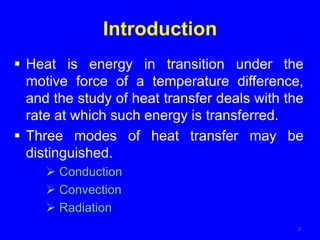
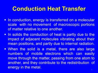
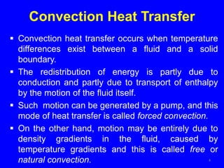
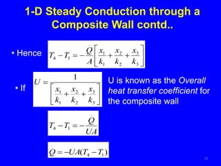
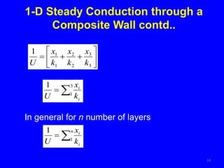
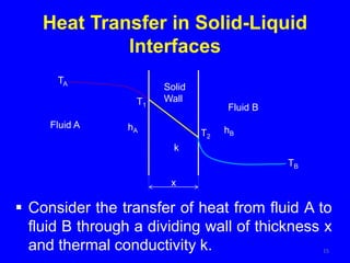
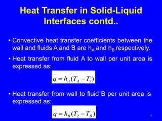
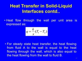
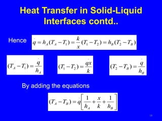
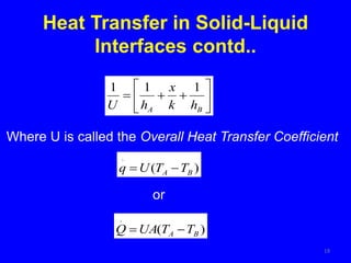
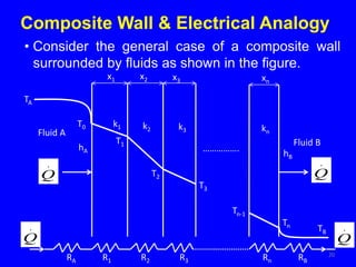
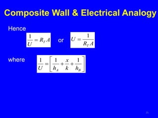
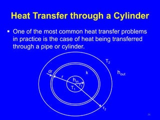
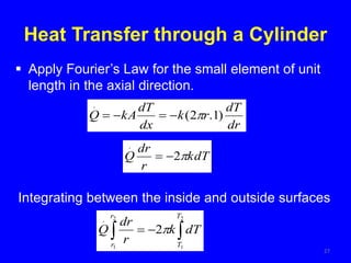
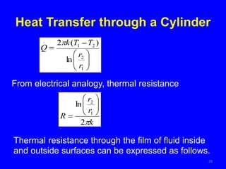
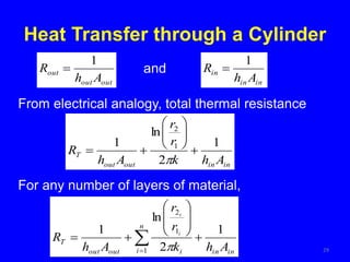
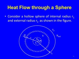
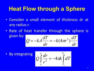
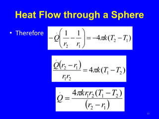
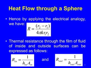
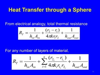
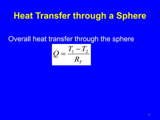
Heat Transfer
Introduction
 Heat is energy in transition under the
motive force of a temperature difference,
and the study of heat transfer deals with the
rate at which such energy is transferred.
 Three modes of heat transfer may be
distinguished.
 Conduction
 Convection
 Radiation
2
Conduction Heat Transfer
 In conduction, energy is transferred on a molecular
scale with no movement of macroscopic portions
of matter relative to one another.
 In solids the conduction of heat is partly due to the
impact of adjacent molecules vibrating about their
mean positions, and partly due to internal radiation.
 When the solid is a metal, there are also large
numbers of mobile electrons which can easily
move through the matter, passing from one atom to
another, and they contribute to the redistribution of
energy in the metal. 3
Convection Heat Transfer
 Convection heat transfer occurs when temperature
differences exist between a fluid and a solid
boundary.
 The redistribution of energy is partly due to
conduction and partly due to transport of enthalpy
by the motion of the fluid itself.
 Such motion can be generated by a pump, and this
mode of heat transfer is called forced convection.
 On the other hand, motion may be entirely due to
density gradients in the fluid, caused by
temperature gradients and this is called free or
natural convection. 4
Radiation Heat Transfer
 Radiation heat transfer does not depend on the
existence of an intervening medium.
 Earth receives energy from the sun through
radiation heat transfer.
 All matters at temperatures above absolute zero
emit heat in the form of electromagnetic waves.
 The calculation of radiation heat transfer is based
mainly on the Stefan-Boltzmann, Kirchhoff and
Lambert Laws.
5
Fourier’s Law of Heat Conduction
6
Fourier’s Law states that the rate of flow of heat
through a single homogeneous solid is
directly proportional to the area (A) of the section
at right angles to the direction of heat flow, and to
the temperature gradient in the direction of heat
flow.
A
Q
.
dx
dT
Q
.
T1 T2
x
dx
Y
Y
dx
dT
A
Q
.
.
Q
.
Q
.
Q
Fourier’s Law of Heat Conduction contd..
7
Hence
dx
dT
kA
Q 

.
k – Constant of proportionality
• k is known as the thermal conductivity of the material
(W/mK).
• Let us consider the transfer of heat through section
Y-Y.
Fourier’s Law of Heat Conduction contd..
8
Hence
dx
dT
kA
Q 

.
or kAdT
dx
Q 

.
By integration

 

2
1
0
.
T
T
x
kAdT
dx
Q
or



2
1
.
T
T
kdT
A
x
Q
Fourier’s Law of Heat Conduction contd..
9
• For most solids, the value of the thermal
conductivity is approximately constant over a
wide range of temperatures and therefore k will be
taken as constant.



2
1
.
T
T
dT
Ak
x
Q or
)
(
)
( 2
1
1
2
.
T
T
x
kA
T
T
x
kA
Q 




1-D Steady Conduction through a
Composite Wall
10
• A wall built up of three different materials is shown
in the figure.
• Surface temperatures of the wall are T1 and T4 and
the temperatures of the interfaces are T2 and T3.
x1 x2 x3
T1
T2
T3
T4
k1 k2 k3
.
Q
.
Q
1-D Steady Conduction through a
Composite Wall contd..
11
• For steady flow through the wall, the heat flow rate
through successive slabs must be the same for the
reasons of continuity, and hence,
)
( 1
2
1
1
.
T
T
x
A
k
Q 


)
( 2
3
2
2
.
T
T
x
A
k
Q 


)
( 3
4
3
3
.
T
T
x
A
k
Q 


1-D Steady Conduction through a
Composite Wall contd..
12
• Hence
A
k
x
Q
T
T
1
1
.
1
2 


A
k
x
Q
T
T
2
2
.
2
3 


A
k
x
Q
T
T
3
3
.
3
4 


• By adding the equations together,
1-D Steady Conduction through a
Composite Wall contd..
13
• Hence 










3
3
2
2
1
1
.
1
4
k
x
k
x
k
x
A
Q
T
T
• If









3
3
2
2
1
1
1
k
x
k
x
k
x
U
UA
Q
T
T
.
1
4 


)
( 1
4
.
T
T
UA
Q 


U is known as the Overall
heat transfer coefficient for
the composite wall
1-D Steady Conduction through a
Composite Wall contd..
14









3
3
2
2
1
1
1
k
x
k
x
k
x
U
In general for n number of layers


3
1
1
i
i
k
x
U


n
i
i
k
x
U 1
1
Heat Transfer in Solid-Liquid
Interfaces
 Consider the transfer of heat from fluid A to
fluid B through a dividing wall of thickness x
and thermal conductivity k. 15
k
hA hB
x
T1
T2
TA
TB
Fluid A
Fluid B
Solid
Wall
16
• Convective heat transfer coefficients between the
wall and fluids A and B are hA and hB respectively.
• Heat transfer from fluid A to wall per unit area is
expressed as:
)
( 1
.
T
T
h
q A
A 

Heat Transfer in Solid-Liquid
Interfaces contd..
• Heat transfer from wall to fluid B per unit area is
expressed as:
)
( 2
.
B
B T
T
h
q 

17
• Heat flow through the wall per unit area is
expressed as:
Heat Transfer in Solid-Liquid
Interfaces contd..
)
( 2
1
.
T
T
x
k
q 

• For steady state heat transfer, the heat flowing
from fluid A to the wall is equal to the heat
flowing through the wall, which is also equal to
the heat flowing from the wall to fluid B.
18
Hence
Heat Transfer in Solid-Liquid
Interfaces contd..
)
(
)
(
)
( 2
2
1
1
.
B
B
A
A T
T
h
T
T
x
k
T
T
h
q 





.
1)
(
A
A
h
q
T
T 

.
2
1 )
(
k
qx
T
T 

.
2 )
(
B
B
h
q
T
T 

By adding the equations










B
A
B
A
h
k
x
h
q
T
T
1
1
)
(
.
19
Heat Transfer in Solid-Liquid
Interfaces contd..
Where U is called the Overall Heat Transfer Coefficient









B
A h
k
x
h
U
1
1
1
)
(
.
B
A T
T
UA
Q 

)
(
.
B
A T
T
U
q 

or
Composite Wall & Electrical Analogy
20
• Consider the general case of a composite wall
surrounded by fluids as shown in the figure.
x1 x2 x3
T0
T1
T2
T3
k1 k2 k3
TA
Fluid A
Fluid B
Tn-1
TB
Tn
kn
xn
…………….
RA R1 R2 R3 Rn RB
.
Q
.
Q
.
Q
.
Q
hA
hB
Composite Wall & Electrical Analogy
21
• The most convenient method of solving such a
problem is by making use of an electrical analogy.
• The flow of heat can be thought of as analogous to
an electric current.
• The heat flow is caused by a temperature difference
whereas the current flow is caused by a potential
difference, hence it is possible to postulate a
thermal resistance analogous to an electrical
resistance.
I
V
R 
Thermal Resistance
kA
x
R 
Composite Wall & Electrical Analogy
22
• is analogous to I and (T1-T2) is analogous to V.
• The composite wall is analogous to a series of
resistances and resistances in series can be
added to give the total resistance.
• Thermal Resistance of the fluid film
A
h
R
i
1

.
Q
A
h
R
A
A
1

A
k
x
R
1
1
1 
A
k
x
R
2
2
2 
A
k
x
R
n
n
n 
A
h
R
B
B
1

Composite Wall & Electrical Analogy
23
Total resistance to heat flow is then,
B
n
A
T R
R
R
R
R
R 




 ....
..........
2
1
A
h
A
k
x
A
k
x
A
h
R
B
n
n
A
T
1
.........
1
1
1





For any number of layers of material,
A
h
A
k
x
A
h
R
B
n
i i
i
A
T
1
1
1


 

Total Resistance
Composite Wall & Electrical Analogy
24
Electrical analogy for the overall heat transfer
For any number of layers
B
n
i i
i
A h
k
x
h
U
1
1
1
1


 

T
B
A
R
T
T
Q


.
It is proved that









B
A h
k
x
h
U
1
1
1
It can be seen that that the reciprocal of U is simply
the thermal resistance for unit area
Composite Wall & Electrical Analogy
25
Hence
A
R
U
T

1
where









B
A h
k
x
h
U
1
1
1
or
A
R
U
T
1

Heat Transfer through a Cylinder
 One of the most common heat transfer problems
in practice is the case of heat being transferred
through a pipe or cylinder.
26
r2
r1
r
T2
T1
dr k hout
hin
Heat Transfer through a Cylinder
 Apply Fourier’s Law for the small element of unit
length in the axial direction.
27
dr
dT
r
k
dx
dT
kA
Q )
1
.
2
(
.





kdT
r
dr
Q 
2
.


Integrating between the inside and outside surfaces

 

2
1
2
1
2
.
T
T
r
r
dT
k
r
dr
Q 
Heat Transfer through a Cylinder
28










1
2
2
1
.
ln
)
(
2
r
r
T
T
k
Q

From electrical analogy, thermal resistance
k
r
r
R

2
ln
1
2









Thermal resistance through the film of fluid inside
and outside surfaces can be expressed as follows.
Heat Transfer through a Cylinder
29
From electrical analogy, total thermal resistance
in
in
out
out
T
A
h
k
r
r
A
h
R
1
2
ln
1 1
2












out
out
out
A
h
R
1

in
in
in
A
h
R
1

and
For any number of layers of material,
in
in
n
i i
out
out
T
A
h
k
r
r
A
h
R i
i
1
2
ln
1
1
1
2










 
 
Heat Transfer through a Cylinder
30
Overall heat transfer through the cylinder
T
R
T
T
Q 2
1
. 

Heat Flow through a Sphere
• Consider a hollow sphere of internal radius r1
and external radius r2 as shown in the figure.
r2
r1
r
T2
T1
dr k
31
hout
hin
Heat Flow through a Sphere
• Consider a small element of thickness dr at
any radius r.
• Rate of heat transfer through the sphere is
given by:
• By integrating
dr
dT
r
k
dr
dT
kA
Q )
4
( 2
.






 

2
1
2
1
4
2
.
T
T
r
r
dT
k
r
dr
Q 
32
Heat Flow through a Sphere
• Therefore
)
(
4
1
1
1
2
1
2
.
T
T
k
r
r
Q 











 
  )
(
4 2
1
2
1
1
2
.
T
T
k
r
r
r
r
Q




 
1
2
2
1
2
1
. )
(
4
r
r
T
T
r
kr
Q




33
Heat Flow through a Sphere
• Hence by applying the electrical analogy,
we have:
• Thermal resistance through the film of fluid
of inside and outside surfaces can be
expressed as follows:
and
34
2
1
1
2
4
)
(
r
kr
r
r
R



in
in
in
A
h
R
1

out
out
out
A
h
R
1

Heat Transfer through a Sphere
35
From electrical analogy, total thermal resistance
out
out
in
in
T
A
h
r
kr
r
r
A
h
R
1
4
)
(
1
2
1
1
2





For any number of layers of material,
out
out
n
i i
in
in
T
A
h
r
r
k
r
r
A
h
R
i
i
i
i
1
4
)
(
1
1 2
1
1
2



 
 
Heat Transfer through a Sphere
36
Overall heat transfer through the sphere
T
R
T
T
Q 2
1
. 

Convection
• This is concerned with the calculation of rates of
heat exchange between fluids and solid
boundaries.
• Main resistance to heat flow from a solid wall to
a fluid is in a comparatively thin boundary layer
adjacent to the wall.
• Within the boundary layer, viscous forces
dominate and main mode of heat transfer is
through conduction.
• Away from the solid wall, pressure forces
dominate and heat transfer is due to convection.37
Flow of fluid over a flat plate
• Fluid flows over a flat plate with a free stream
velocity Us.
• Fluid velocity adjacent to the surface of plate is
zero.
• There is no-slip between fluid and solid surface.
• In the direction perpendicular to the plate, the
stream velocity increases and approaches the
free stream velocity.
• The two regions in fluid, both boundary layer
and free stream is shown in the figure below:
38
Flow of fluid over a flat plate
39
Free Stream
Flow of fluid over a flat plate
• If the flow approaching the leading edge of the
plate is laminar, a laminar boundary layer of
thickness δ builds up on the plate.
• At the edge of the plate δ is zero and it
increases gradually with the distance x.
• The shear stress at any point in the fluid is
given by:
40










dy
dU

 where μ is the dynamic
viscosity
Flow of fluid over a flat plate
• Thickness of the boundary layer increases with
the distance x from the leading edge of the plate
according to:
41
  5
.
0
Re
64
.
4
x
x


where Rex is the Reynolds number based on the
distance x:

 x
U s
x 
Re
Flow of fluid over a flat plate
• The shear stress at the wall is expressed as:
• The average friction factor f is found to be:
• Beyond a certain critical distance xcr, from the
leading edge, the flow becomes fully turbulent
as shown below: 42
where f is the dimensionless
friction factor
2
2
s
w
U
f

 
w

  5
.
0
Re
328
.
1
x
f 
Flow of fluid over a flat plate
• The critical distance, in terms of the Reynolds
number is found from experiments as:
43
Us
Us
Us
cr
s
cr
U
x Re


 where Recr = 500,000
Radiation Heat Transfer
 Any matter with temperature above absolute
zero (0 K) emits electromagnetic radiation
 Intensity of radiant energy flux depends upon
the temperature of the body and the nature
of its surface
 Radiation heat transfer does not need a
medium
 In order to understand radiation heat transfer,
study of electro-magnetic spectrum is needed
44
Electromagnetic Spectrum
45
Black Body Radiation
 A black body absorbs all energy that reaches it
completely
 It is also a perfect emitter
46
Radiative Properties
 When radiation strikes a surface, a portion of it is
reflected, and the rest penetrates the surface
 Out of the radiation that enters the object, some
proportion is absorbed by the material, and the rest
is transmitted through
47
Radiative Properties contd..
 The ratio of reflected energy to the incident energy
is called Reflectivity (ρ)
 Transmissivity (τ) is defined as the fraction of the
incident energy that is transmitted through the
object
 Absorptivity (α) is defined as the fraction of the
incident energy that is absorbed by the object
 Hence,
 All three radiative properties have typical values
between 0 and 1
48
1


 


Stefan-Boltzmann Law
• The radiant energy emitted by a blackbody per
unit time can be determined from the Stefan-
Boltzmann Law:
49
4
.
AT
Q 
 where
- Blackbody emissive power (W)
A - Surface area (m2)
T - Absolute temperature of the surface (K)
σ - Stefan-Boltzmann constant (5.67 x 10⁻⁸ W/m2K4)
.
Q
Emissive Power
50
Emissivity (ε)
 Emissivity is the ratio of a surface's ability to emit
radiant energy compared with the ability of a perfect
black body of the same area at the same
temperature
 Emissivity is a dimensionless constant having values
between 0 and 1
 A material with high emissivity is efficient in both
absorbing radiant energy as well as emitting it
 Therefore, a good absorber is also a good emitter
51
4
.
AT
Q 
 ε – Emissivity of surface
Grey Body
 A Grey body has a constant emissivity over all
wavelengths and for all temperatures
 For a grey body at all temperatures,
where α and ε are total absorptivity and the
total emissivity over all wavelengths
52

 
Radiation Exchange
 Consider a body of emissivity ε at a temperature
T1, completely surrounded by black surroundings
at a lower temperature T2.
 Energy leaving the body is completely absorbed
by the surroundings, where rate of radiant energy
emission per unit area =
 Rate of energy emitted by the black surroundings
per unit area =
 Fraction of this energy which is absorbed by the
body depends on the absorptivity of the same
53
4
1
T

4
2
T

Radiation Exchange contd..
 For a grey body at all temperatures and
hence:
Rate of energy absorption =
 Hence, rate of heat transferred from the body
to its surroundings per unit area is:
54

 
4
2
4
2 T
T 
 
 
4
2
4
1
4
2
4
1
.
T
T
T
T
q 


 


Net Radiant Heat Transfer between
Surfaces
55
Net Radiant Heat Transfer between
Surfaces contd..
 Figure shows two arbitrary surfaces exchanging radiant
energy between them
 If surfaces are “black” then the net radiant energy
exchanged:
 View factor is purely a geometrical parameter (ranges
between 0 and 1) that accounts for the effect of
orientation on radiant heat exchange between surfaces
 Furthermore or
56
 
4
2
4
1
12
.
T
T
A
F
Qnet 
  where
F12 - View factor (Shape factor) between the surfaces
21
2
12
1 F
A
F
A  ji
j
ij
i F
A
F
A 
Radiant heat transfer between
surfaces
 Radiant heat exchange between two surfaces is given
by:
 View factor is purely a geometrical parameter that
accounts for the effect of orientation on radiant heat
exchange between surfaces.
 The view factor ranges between 0 and 1
57
 
4
4
.
cold
cold
hot
hot T
T
AF
Q 

 
 where
F - View factor (Shape factor) between surfaces

Heat Transfer and mass trtransfer lecture

  • 1.
  • 2.
    Introduction  Heat isenergy in transition under the motive force of a temperature difference, and the study of heat transfer deals with the rate at which such energy is transferred.  Three modes of heat transfer may be distinguished.  Conduction  Convection  Radiation 2
  • 3.
    Conduction Heat Transfer In conduction, energy is transferred on a molecular scale with no movement of macroscopic portions of matter relative to one another.  In solids the conduction of heat is partly due to the impact of adjacent molecules vibrating about their mean positions, and partly due to internal radiation.  When the solid is a metal, there are also large numbers of mobile electrons which can easily move through the matter, passing from one atom to another, and they contribute to the redistribution of energy in the metal. 3
  • 4.
    Convection Heat Transfer Convection heat transfer occurs when temperature differences exist between a fluid and a solid boundary.  The redistribution of energy is partly due to conduction and partly due to transport of enthalpy by the motion of the fluid itself.  Such motion can be generated by a pump, and this mode of heat transfer is called forced convection.  On the other hand, motion may be entirely due to density gradients in the fluid, caused by temperature gradients and this is called free or natural convection. 4
  • 5.
    Radiation Heat Transfer Radiation heat transfer does not depend on the existence of an intervening medium.  Earth receives energy from the sun through radiation heat transfer.  All matters at temperatures above absolute zero emit heat in the form of electromagnetic waves.  The calculation of radiation heat transfer is based mainly on the Stefan-Boltzmann, Kirchhoff and Lambert Laws. 5
  • 6.
    Fourier’s Law ofHeat Conduction 6 Fourier’s Law states that the rate of flow of heat through a single homogeneous solid is directly proportional to the area (A) of the section at right angles to the direction of heat flow, and to the temperature gradient in the direction of heat flow. A Q . dx dT Q . T1 T2 x dx Y Y dx dT A Q . . Q . Q . Q
  • 7.
    Fourier’s Law ofHeat Conduction contd.. 7 Hence dx dT kA Q   . k – Constant of proportionality • k is known as the thermal conductivity of the material (W/mK). • Let us consider the transfer of heat through section Y-Y.
  • 8.
    Fourier’s Law ofHeat Conduction contd.. 8 Hence dx dT kA Q   . or kAdT dx Q   . By integration     2 1 0 . T T x kAdT dx Q or    2 1 . T T kdT A x Q
  • 9.
    Fourier’s Law ofHeat Conduction contd.. 9 • For most solids, the value of the thermal conductivity is approximately constant over a wide range of temperatures and therefore k will be taken as constant.    2 1 . T T dT Ak x Q or ) ( ) ( 2 1 1 2 . T T x kA T T x kA Q     
  • 10.
    1-D Steady Conductionthrough a Composite Wall 10 • A wall built up of three different materials is shown in the figure. • Surface temperatures of the wall are T1 and T4 and the temperatures of the interfaces are T2 and T3. x1 x2 x3 T1 T2 T3 T4 k1 k2 k3 . Q . Q
  • 11.
    1-D Steady Conductionthrough a Composite Wall contd.. 11 • For steady flow through the wall, the heat flow rate through successive slabs must be the same for the reasons of continuity, and hence, ) ( 1 2 1 1 . T T x A k Q    ) ( 2 3 2 2 . T T x A k Q    ) ( 3 4 3 3 . T T x A k Q   
  • 12.
    1-D Steady Conductionthrough a Composite Wall contd.. 12 • Hence A k x Q T T 1 1 . 1 2    A k x Q T T 2 2 . 2 3    A k x Q T T 3 3 . 3 4    • By adding the equations together,
  • 13.
    1-D Steady Conductionthrough a Composite Wall contd.. 13 • Hence            3 3 2 2 1 1 . 1 4 k x k x k x A Q T T • If          3 3 2 2 1 1 1 k x k x k x U UA Q T T . 1 4    ) ( 1 4 . T T UA Q    U is known as the Overall heat transfer coefficient for the composite wall
  • 14.
    1-D Steady Conductionthrough a Composite Wall contd.. 14          3 3 2 2 1 1 1 k x k x k x U In general for n number of layers   3 1 1 i i k x U   n i i k x U 1 1
  • 15.
    Heat Transfer inSolid-Liquid Interfaces  Consider the transfer of heat from fluid A to fluid B through a dividing wall of thickness x and thermal conductivity k. 15 k hA hB x T1 T2 TA TB Fluid A Fluid B Solid Wall
  • 16.
    16 • Convective heattransfer coefficients between the wall and fluids A and B are hA and hB respectively. • Heat transfer from fluid A to wall per unit area is expressed as: ) ( 1 . T T h q A A   Heat Transfer in Solid-Liquid Interfaces contd.. • Heat transfer from wall to fluid B per unit area is expressed as: ) ( 2 . B B T T h q  
  • 17.
    17 • Heat flowthrough the wall per unit area is expressed as: Heat Transfer in Solid-Liquid Interfaces contd.. ) ( 2 1 . T T x k q   • For steady state heat transfer, the heat flowing from fluid A to the wall is equal to the heat flowing through the wall, which is also equal to the heat flowing from the wall to fluid B.
  • 18.
    18 Hence Heat Transfer inSolid-Liquid Interfaces contd.. ) ( ) ( ) ( 2 2 1 1 . B B A A T T h T T x k T T h q       . 1) ( A A h q T T   . 2 1 ) ( k qx T T   . 2 ) ( B B h q T T   By adding the equations           B A B A h k x h q T T 1 1 ) ( .
  • 19.
    19 Heat Transfer inSolid-Liquid Interfaces contd.. Where U is called the Overall Heat Transfer Coefficient          B A h k x h U 1 1 1 ) ( . B A T T UA Q   ) ( . B A T T U q   or
  • 20.
    Composite Wall &Electrical Analogy 20 • Consider the general case of a composite wall surrounded by fluids as shown in the figure. x1 x2 x3 T0 T1 T2 T3 k1 k2 k3 TA Fluid A Fluid B Tn-1 TB Tn kn xn ……………. RA R1 R2 R3 Rn RB . Q . Q . Q . Q hA hB
  • 21.
    Composite Wall &Electrical Analogy 21 • The most convenient method of solving such a problem is by making use of an electrical analogy. • The flow of heat can be thought of as analogous to an electric current. • The heat flow is caused by a temperature difference whereas the current flow is caused by a potential difference, hence it is possible to postulate a thermal resistance analogous to an electrical resistance. I V R  Thermal Resistance kA x R 
  • 22.
    Composite Wall &Electrical Analogy 22 • is analogous to I and (T1-T2) is analogous to V. • The composite wall is analogous to a series of resistances and resistances in series can be added to give the total resistance. • Thermal Resistance of the fluid film A h R i 1  . Q A h R A A 1  A k x R 1 1 1  A k x R 2 2 2  A k x R n n n  A h R B B 1 
  • 23.
    Composite Wall &Electrical Analogy 23 Total resistance to heat flow is then, B n A T R R R R R R       .... .......... 2 1 A h A k x A k x A h R B n n A T 1 ......... 1 1 1      For any number of layers of material, A h A k x A h R B n i i i A T 1 1 1      Total Resistance
  • 24.
    Composite Wall &Electrical Analogy 24 Electrical analogy for the overall heat transfer For any number of layers B n i i i A h k x h U 1 1 1 1      T B A R T T Q   . It is proved that          B A h k x h U 1 1 1 It can be seen that that the reciprocal of U is simply the thermal resistance for unit area
  • 25.
    Composite Wall &Electrical Analogy 25 Hence A R U T  1 where          B A h k x h U 1 1 1 or A R U T 1 
  • 26.
    Heat Transfer througha Cylinder  One of the most common heat transfer problems in practice is the case of heat being transferred through a pipe or cylinder. 26 r2 r1 r T2 T1 dr k hout hin
  • 27.
    Heat Transfer througha Cylinder  Apply Fourier’s Law for the small element of unit length in the axial direction. 27 dr dT r k dx dT kA Q ) 1 . 2 ( .      kdT r dr Q  2 .   Integrating between the inside and outside surfaces     2 1 2 1 2 . T T r r dT k r dr Q 
  • 28.
    Heat Transfer througha Cylinder 28           1 2 2 1 . ln ) ( 2 r r T T k Q  From electrical analogy, thermal resistance k r r R  2 ln 1 2          Thermal resistance through the film of fluid inside and outside surfaces can be expressed as follows.
  • 29.
    Heat Transfer througha Cylinder 29 From electrical analogy, total thermal resistance in in out out T A h k r r A h R 1 2 ln 1 1 2             out out out A h R 1  in in in A h R 1  and For any number of layers of material, in in n i i out out T A h k r r A h R i i 1 2 ln 1 1 1 2              
  • 30.
    Heat Transfer througha Cylinder 30 Overall heat transfer through the cylinder T R T T Q 2 1 .  
  • 31.
    Heat Flow througha Sphere • Consider a hollow sphere of internal radius r1 and external radius r2 as shown in the figure. r2 r1 r T2 T1 dr k 31 hout hin
  • 32.
    Heat Flow througha Sphere • Consider a small element of thickness dr at any radius r. • Rate of heat transfer through the sphere is given by: • By integrating dr dT r k dr dT kA Q ) 4 ( 2 .          2 1 2 1 4 2 . T T r r dT k r dr Q  32
  • 33.
    Heat Flow througha Sphere • Therefore ) ( 4 1 1 1 2 1 2 . T T k r r Q                 ) ( 4 2 1 2 1 1 2 . T T k r r r r Q       1 2 2 1 2 1 . ) ( 4 r r T T r kr Q     33
  • 34.
    Heat Flow througha Sphere • Hence by applying the electrical analogy, we have: • Thermal resistance through the film of fluid of inside and outside surfaces can be expressed as follows: and 34 2 1 1 2 4 ) ( r kr r r R    in in in A h R 1  out out out A h R 1 
  • 35.
    Heat Transfer througha Sphere 35 From electrical analogy, total thermal resistance out out in in T A h r kr r r A h R 1 4 ) ( 1 2 1 1 2      For any number of layers of material, out out n i i in in T A h r r k r r A h R i i i i 1 4 ) ( 1 1 2 1 1 2       
  • 36.
    Heat Transfer througha Sphere 36 Overall heat transfer through the sphere T R T T Q 2 1 .  
  • 37.
    Convection • This isconcerned with the calculation of rates of heat exchange between fluids and solid boundaries. • Main resistance to heat flow from a solid wall to a fluid is in a comparatively thin boundary layer adjacent to the wall. • Within the boundary layer, viscous forces dominate and main mode of heat transfer is through conduction. • Away from the solid wall, pressure forces dominate and heat transfer is due to convection.37
  • 38.
    Flow of fluidover a flat plate • Fluid flows over a flat plate with a free stream velocity Us. • Fluid velocity adjacent to the surface of plate is zero. • There is no-slip between fluid and solid surface. • In the direction perpendicular to the plate, the stream velocity increases and approaches the free stream velocity. • The two regions in fluid, both boundary layer and free stream is shown in the figure below: 38
  • 39.
    Flow of fluidover a flat plate 39 Free Stream
  • 40.
    Flow of fluidover a flat plate • If the flow approaching the leading edge of the plate is laminar, a laminar boundary layer of thickness δ builds up on the plate. • At the edge of the plate δ is zero and it increases gradually with the distance x. • The shear stress at any point in the fluid is given by: 40           dy dU   where μ is the dynamic viscosity
  • 41.
    Flow of fluidover a flat plate • Thickness of the boundary layer increases with the distance x from the leading edge of the plate according to: 41   5 . 0 Re 64 . 4 x x   where Rex is the Reynolds number based on the distance x:   x U s x  Re
  • 42.
    Flow of fluidover a flat plate • The shear stress at the wall is expressed as: • The average friction factor f is found to be: • Beyond a certain critical distance xcr, from the leading edge, the flow becomes fully turbulent as shown below: 42 where f is the dimensionless friction factor 2 2 s w U f    w    5 . 0 Re 328 . 1 x f 
  • 43.
    Flow of fluidover a flat plate • The critical distance, in terms of the Reynolds number is found from experiments as: 43 Us Us Us cr s cr U x Re    where Recr = 500,000
  • 44.
    Radiation Heat Transfer Any matter with temperature above absolute zero (0 K) emits electromagnetic radiation  Intensity of radiant energy flux depends upon the temperature of the body and the nature of its surface  Radiation heat transfer does not need a medium  In order to understand radiation heat transfer, study of electro-magnetic spectrum is needed 44
  • 45.
  • 46.
    Black Body Radiation A black body absorbs all energy that reaches it completely  It is also a perfect emitter 46
  • 47.
    Radiative Properties  Whenradiation strikes a surface, a portion of it is reflected, and the rest penetrates the surface  Out of the radiation that enters the object, some proportion is absorbed by the material, and the rest is transmitted through 47
  • 48.
    Radiative Properties contd.. The ratio of reflected energy to the incident energy is called Reflectivity (ρ)  Transmissivity (τ) is defined as the fraction of the incident energy that is transmitted through the object  Absorptivity (α) is defined as the fraction of the incident energy that is absorbed by the object  Hence,  All three radiative properties have typical values between 0 and 1 48 1      
  • 49.
    Stefan-Boltzmann Law • Theradiant energy emitted by a blackbody per unit time can be determined from the Stefan- Boltzmann Law: 49 4 . AT Q   where - Blackbody emissive power (W) A - Surface area (m2) T - Absolute temperature of the surface (K) σ - Stefan-Boltzmann constant (5.67 x 10⁻⁸ W/m2K4) . Q
  • 50.
  • 51.
    Emissivity (ε)  Emissivityis the ratio of a surface's ability to emit radiant energy compared with the ability of a perfect black body of the same area at the same temperature  Emissivity is a dimensionless constant having values between 0 and 1  A material with high emissivity is efficient in both absorbing radiant energy as well as emitting it  Therefore, a good absorber is also a good emitter 51 4 . AT Q   ε – Emissivity of surface
  • 52.
    Grey Body  AGrey body has a constant emissivity over all wavelengths and for all temperatures  For a grey body at all temperatures, where α and ε are total absorptivity and the total emissivity over all wavelengths 52   
  • 53.
    Radiation Exchange  Considera body of emissivity ε at a temperature T1, completely surrounded by black surroundings at a lower temperature T2.  Energy leaving the body is completely absorbed by the surroundings, where rate of radiant energy emission per unit area =  Rate of energy emitted by the black surroundings per unit area =  Fraction of this energy which is absorbed by the body depends on the absorptivity of the same 53 4 1 T  4 2 T 
  • 54.
    Radiation Exchange contd.. For a grey body at all temperatures and hence: Rate of energy absorption =  Hence, rate of heat transferred from the body to its surroundings per unit area is: 54    4 2 4 2 T T      4 2 4 1 4 2 4 1 . T T T T q       
  • 55.
    Net Radiant HeatTransfer between Surfaces 55
  • 56.
    Net Radiant HeatTransfer between Surfaces contd..  Figure shows two arbitrary surfaces exchanging radiant energy between them  If surfaces are “black” then the net radiant energy exchanged:  View factor is purely a geometrical parameter (ranges between 0 and 1) that accounts for the effect of orientation on radiant heat exchange between surfaces  Furthermore or 56   4 2 4 1 12 . T T A F Qnet    where F12 - View factor (Shape factor) between the surfaces 21 2 12 1 F A F A  ji j ij i F A F A 
  • 57.
    Radiant heat transferbetween surfaces  Radiant heat exchange between two surfaces is given by:  View factor is purely a geometrical parameter that accounts for the effect of orientation on radiant heat exchange between surfaces.  The view factor ranges between 0 and 1 57   4 4 . cold cold hot hot T T AF Q      where F - View factor (Shape factor) between surfaces