Heat transfer chapter 2.pdf best of all u can use it

1. CHAPTER TWO
ONE DIMENSTIONAL HEAT
CONDUCTION
Adama Science and Technology
University
Heat Transfer (MEng3208)

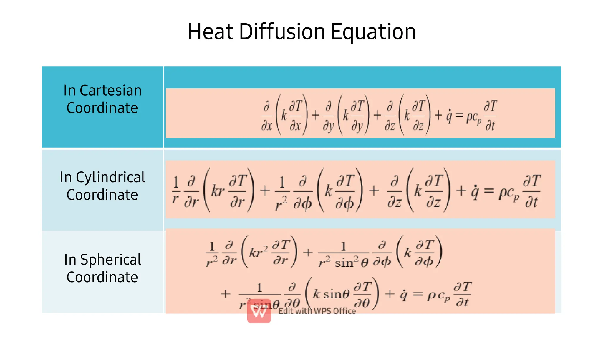
2. 2.1 The Heat Diffusion Equation
•
•
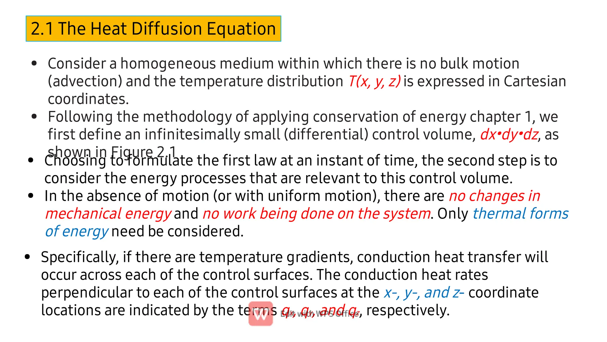
Consider a homogeneous medium within which there is no bulk motion
(advection) and the temperature distribution T(x, y, z) is expressed in Cartesian
coordinates.
Following the methodology of applying conservation of energy chapter 1, we
first define an infinitesimally small (differential) control volume, dxꞏdyꞏdz, as
shown in Figure 2.1
•
•
Choosing to formulate the first law at an instant of time, the second step is to
consider the energy processes that are relevant to this control volume.
In the absence of motion (or with uniform motion), there are no changes in
mechanical energy and no work being done on the system. Only thermal forms
of energy need be considered.
• Specifically, if there are temperature gradients, conduction heat transfer will
occur across each of the control surfaces. The conduction heat rates
perpendicular to each of the control surfaces at the x-, y-, and z- coordinate
locations are indicated by the terms qx, qy, and qz, respectively.

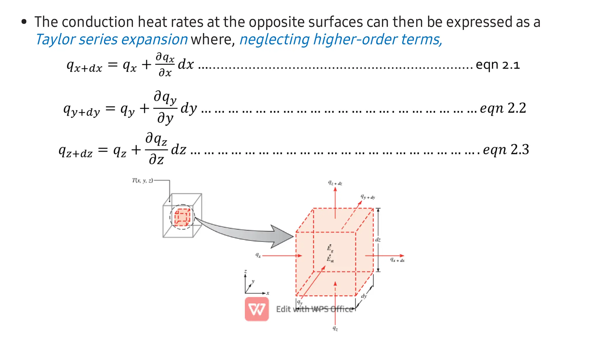
3. • The conduction heat rates at the opposite surfaces can then be expressed as a
Taylor series expansion where, neglecting higher-order terms,

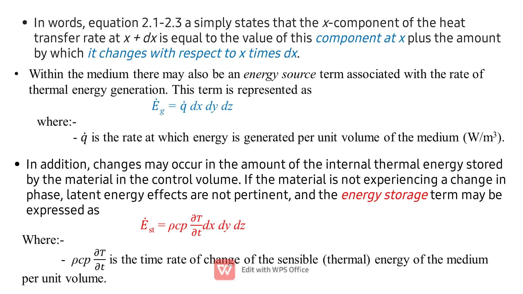
4. • In words, equation 2.1-2.3 a simply states that the x-component of the heat
transfer rate at x + dx is equal to the value of this component at x plus the amount
by which it changes with respect to x times dx.
• In addition, changes may occur in the amount of the internal thermal energy stored
by the material in the control volume. If the material is not experiencing a change in
phase, latent energy effects are not pertinent, and the energy storage term may be
expressed as

5. In Cartesian
Coordinate
In Cylindrical
Coordinate
In Spherical
Coordinate
Heat Diffusion Equation

6. Simplified Heat Diffusion Equation Derivation

8. Boundary and Initial
Conditions
•
•
•
•
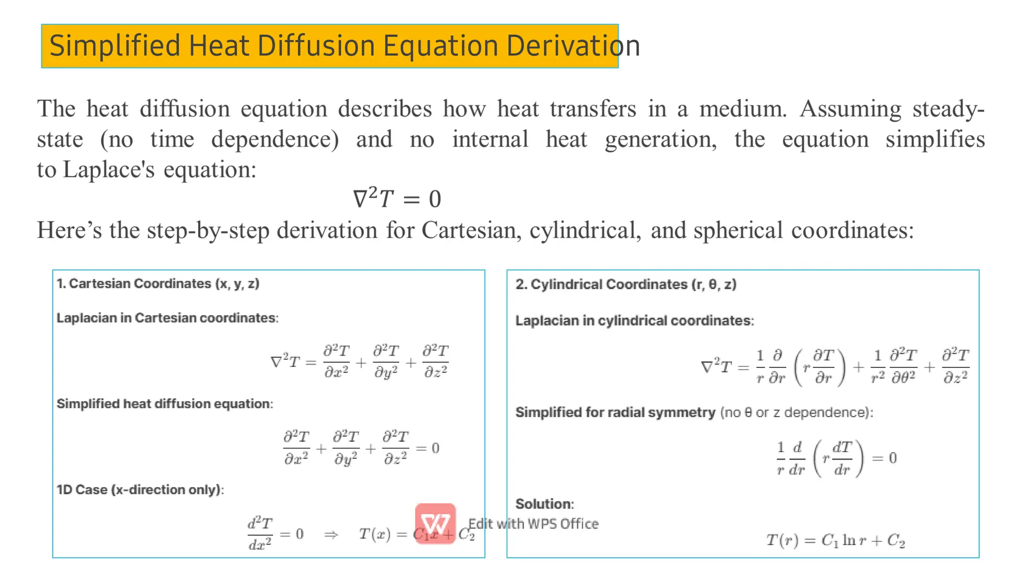
To determine the temperature distribution in a medium, it is necessary to
solve the appropriate form of the heat equation.
However, such a solution depends on the physical conditions existing at the
boundaries of the medium and, if the situation is time dependent, on
conditions existing in the medium at some initial time.
With regard to the boundary conditions, there are several common
possibilities that are simply expressed in mathematical form. Because the
heat equation is second order in the spatial coordinates, two boundary
conditions must be expressed for each coordinate needed to describe the
system.
Because the equation is first order in time, however, only one condition,
termed the initial condition, must be specified.
Types of Boundary and Initial
Conditions

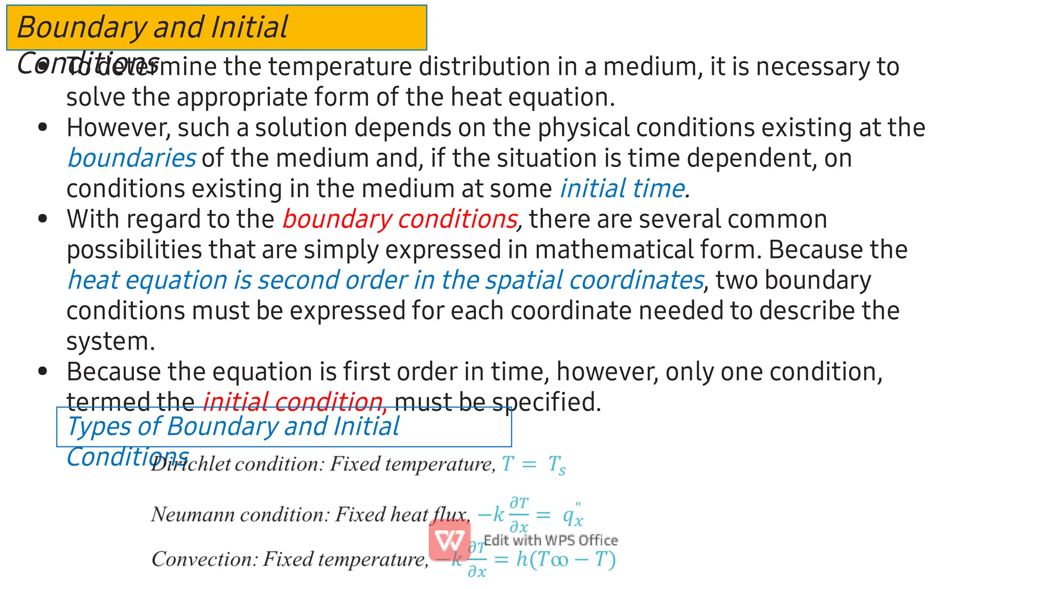
9. • For one-dimensional, steady-state
conduction in a plane wall with no heat
generation and constant thermal
conductivity, the temperature varies linearly
with x.
• For steady-state conditions with no heat
generation, the appropriate form of the
heat equation,
• The rate at which energy is conducted
across any cylindrical surface in the solid
may be expressed as

10. 2.2 The Plane
Wall
•
•
•
•
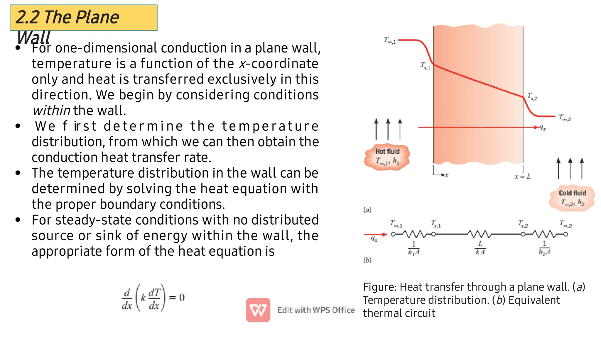
For one-dimensional conduction in a plane wall,
temperature is a function of the x-coordinate
only and heat is transferred exclusively in this
direction. We begin by considering conditions
within the wall.
We f ir st de te r mi ne th e te mpe rature
distribution, from which we can then obtain the
conduction heat transfer rate.
The temperature distribution in the wall can be
determined by solving the heat equation with
the proper boundary conditions.
For steady-state conditions with no distributed
source or sink of energy within the wall, the
appropriate form of the heat equation is
Figure: Heat transfer through a plane wall. (a)
Temperature distribution. (b) Equivalent
thermal circuit

11. 1.3 Thermal Resistance & Overall heat transfer coefficient (U)
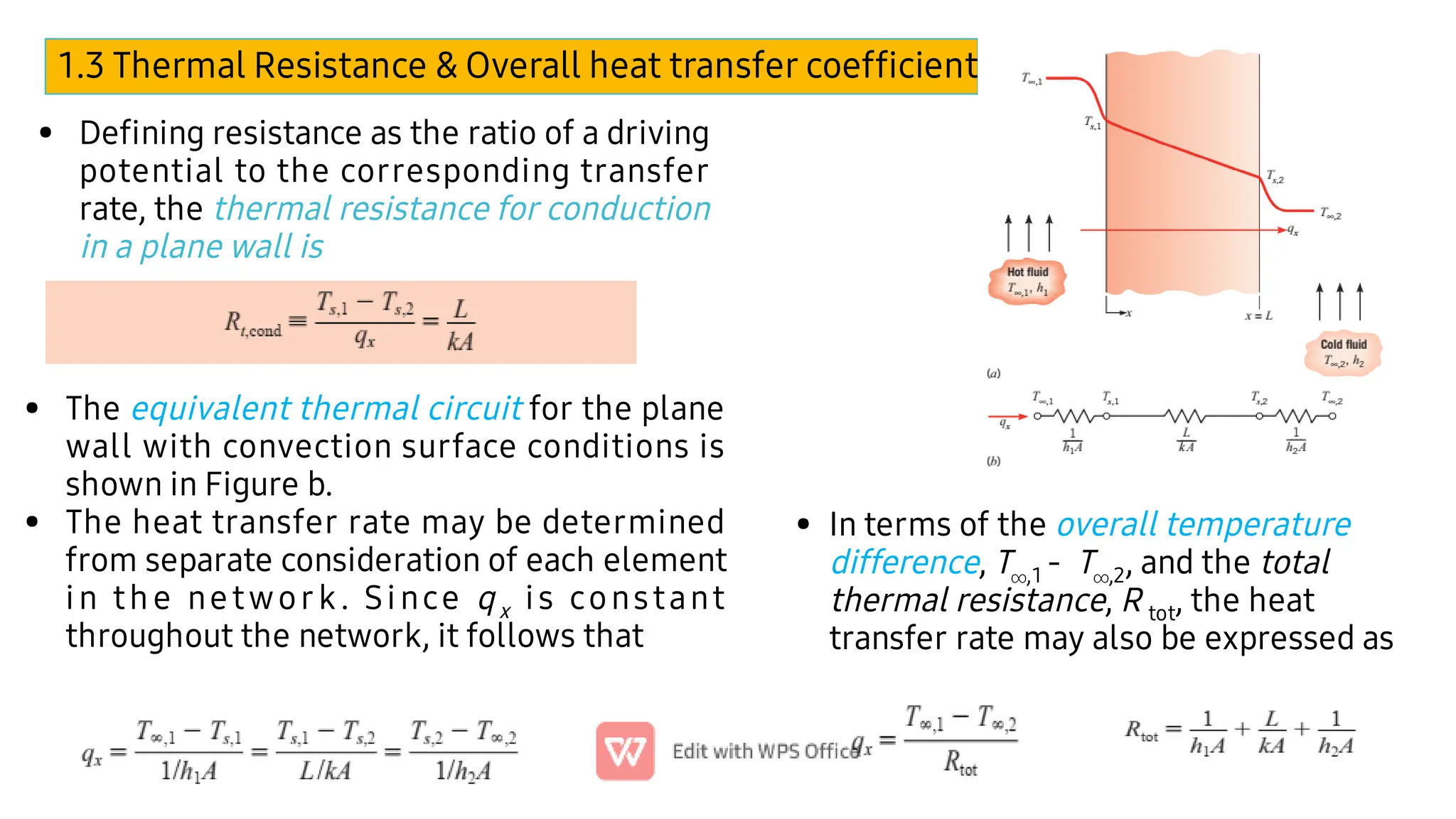
• Defining resistance as the ratio of a driving
potential to the corresponding transfer
rate, the thermal resistance for conduction
in a plane wall is
•
•
The equivalent thermal circuit for the plane
wall with convection surface conditions is
shown in Figure b.
The heat transfer rate may be determined
from separate consideration of each element
in the network. Since qx is constant
throughout the network, it follows that
• In terms of the overall temperature
difference, T,1 - T,2, and the total
thermal resistance, R tot, the heat
transfer rate may also be expressed as

12. The Composite Wall
•
•
•
•
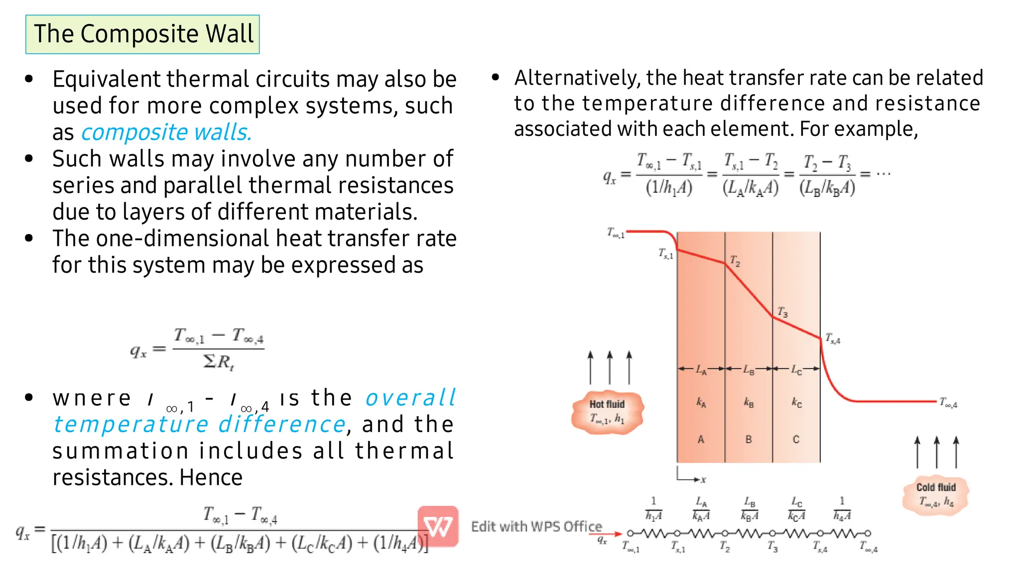
Equivalent thermal circuits may also be
used for more complex systems, such
as composite walls.
Such walls may involve any number of
series and parallel thermal resistances
due to layers of different materials.
The one-dimensional heat transfer rate
for this system may be expressed as
wh e re T  , 1 - T , 4 is th e overall
temperature difference, and the
summation includes all thermal
resistances. Hence
• Alternatively, the heat transfer rate can be related
to the temperature difference and resistance
associated with each element. For example,

14. Reading assignment
Contact Resistance

15. Radial Systems
•
•
•
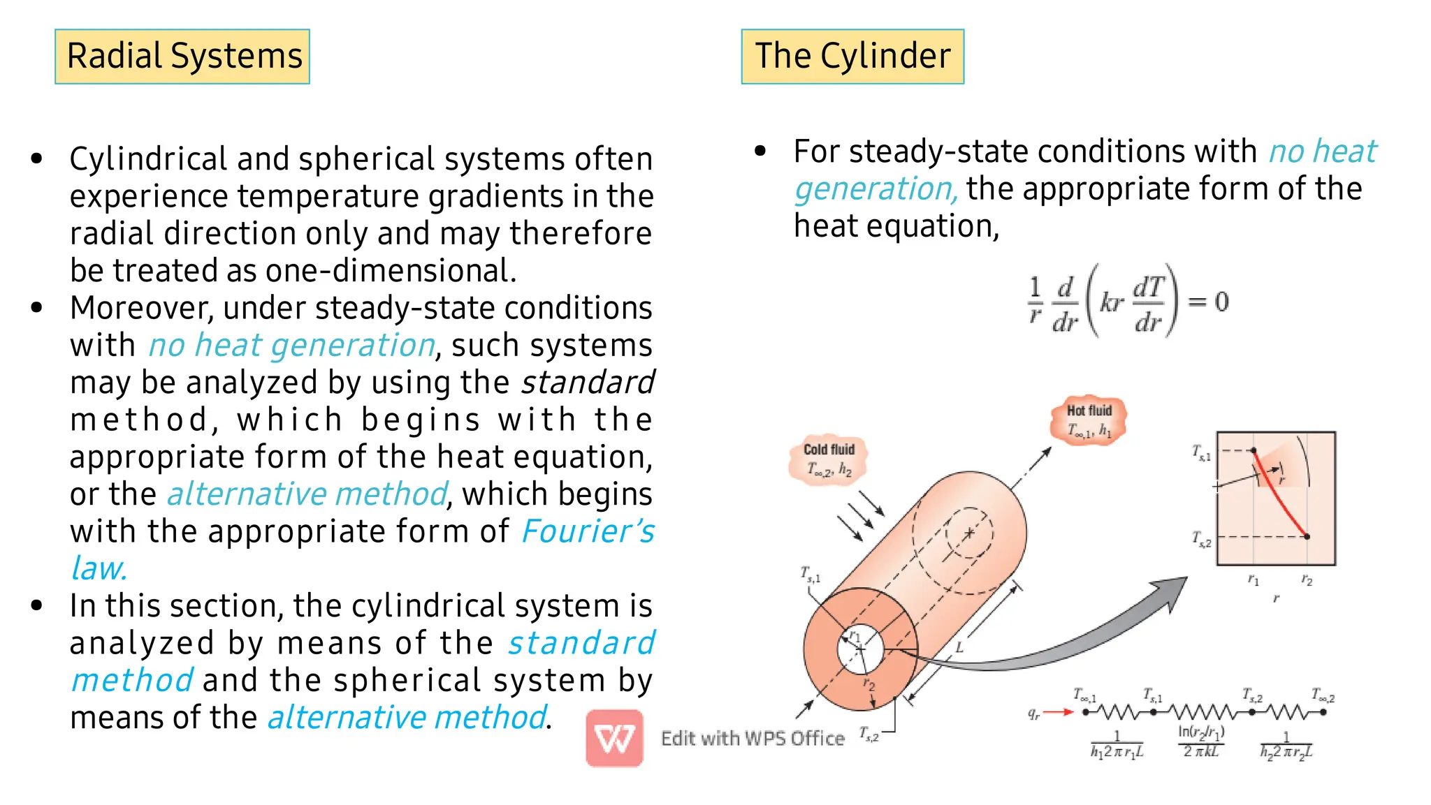
Cylindrical and spherical systems often
experience temperature gradients in the
radial direction only and may therefore
be treated as one-dimensional.
Moreover, under steady-state conditions
with no heat generation, such systems
may be analyzed by using the standard
me th od, w h i ch be gi ns w i th th e
appropriate form of the heat equation,
or the alternative method, which begins
with the appropriate form of Fourier’s
law.
In this section, the cylindrical system is
analyzed by means of the standard
method and the spherical system by
means of the alternative method.
The Cylinder
• For steady-state conditions with no heat
generation, the appropriate form of the
heat equation,

16. •
•
•
•
•
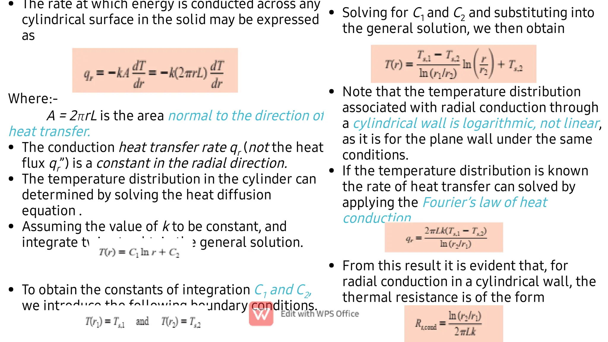
The rate at which energy is conducted across any
cylindrical surface in the solid may be expressed
as
Where:-
A = 2rL is the area normal to the direction of
heat transfer.
The conduction heat transfer rate qr (not the heat
flux qr”) is a constant in the radial direction.
The temperature distribution in the cylinder can
determined by solving the heat diffusion
equation .
Assuming the value of k to be constant, and
integrate twice to obtain the general solution.
To obtain the constants of integration C1 and C2,
we introduce the following boundary conditions.
•
•
•
•
Solving for C1 and C2 and substituting into
the general solution, we then obtain
Note that the temperature distribution
associated with radial conduction through
a cylindrical wall is logarithmic, not linear,
as it is for the plane wall under the same
conditions.
If the temperature distribution is known
the rate of heat transfer can solved by
applying the Fourier’s law of heat
conduction.
From this result it is evident that, for
radial conduction in a cylindrical wall, the
thermal resistance is of the form

17. The composite material
•
•
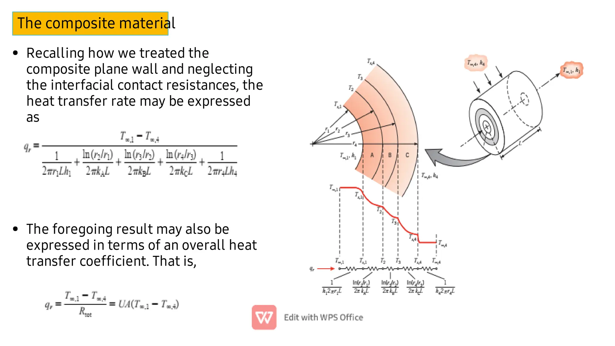
Recalling how we treated the
composite plane wall and neglecting
the interfacial contact resistances, the
heat transfer rate may be expressed
as
The foregoing result may also be
expressed in terms of an overall heat
transfer coefficient. That is,

18. Reading assignment
The sphere

19. Summary of One-Dimensional Conduction Results

20. Conduction with thermal energy generation
•
•
•
•
In the preceding section we considered
conduction problems for which the
temperature distribution in a medium was
determined solely by conditions at the
boundaries of the medium.
We now want to consider the additional effect
on the temperature distribution of processes
that may be occurring within the medium.
In particular, we wish to consider situations for
which thermal energy is being generated due
to conversion from some other energy form.
A common thermal energy generation process
involves the conversion from electrical to
thermal energy in a current-carrying medium
(Ohmic, or resistance, or Joule heating).
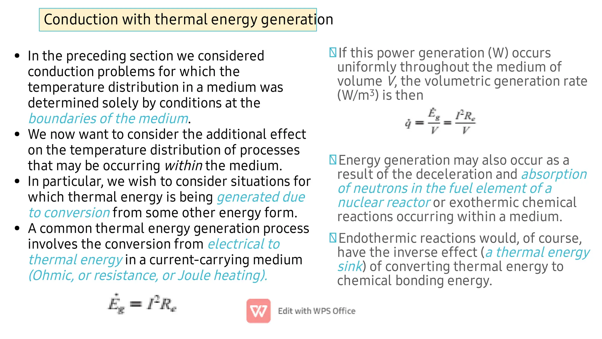
If this power generation (W) occurs
uniformly throughout the medium of
volume V, the volumetric generation rate
(W/m3) is then
Energy generation may also occur as a
result of the deceleration and absorption
of neutrons in the fuel element of a
nuclear reactor or exothermic chemical
reactions occurring within a medium.
Endothermic reactions would, of course,
have the inverse effect (a thermal energy
sink) of converting thermal energy to
chemical bonding energy.

21. The Plane Wall
•
•
•
For constant thermal conductivity k,
the appropriate form of the heat
equation,
The general solution is
where C1 and C2 are the constants of
integration. For the prescribed boundary
conditions,
The constants may be evaluated and
are of the form
•
•
•
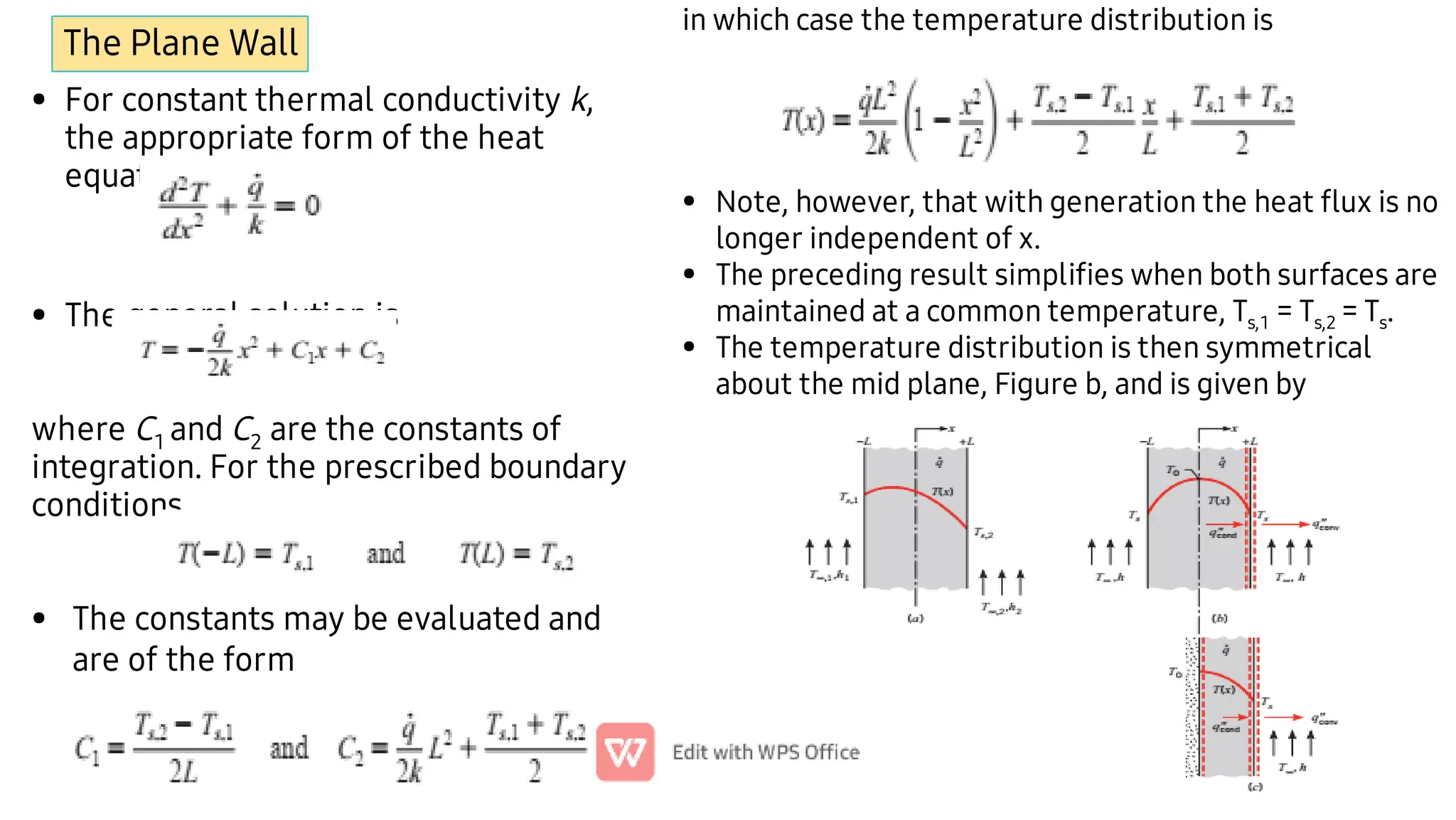
in which case the temperature distribution is
Note, however, that with generation the heat flux is no
longer independent of x.
The preceding result simplifies when both surfaces are
maintained at a common temperature, Ts,1 = Ts,2 = Ts.
The temperature distribution is then symmetrical
about the mid plane, Figure b, and is given by

22. •
•
•
•
The maximum temperature exists at the mid
plane
Rearranging for T(x)
It is important to note that at the plane of
symmetry in Figure b, the temperature gradient
is zero, (dT/dx)x=0 = 0.
Accordingly, there is no heat transfer across this
plane, and it may be represented by the
adiabatic surface shown in Figure c.
•
•
•
•
•
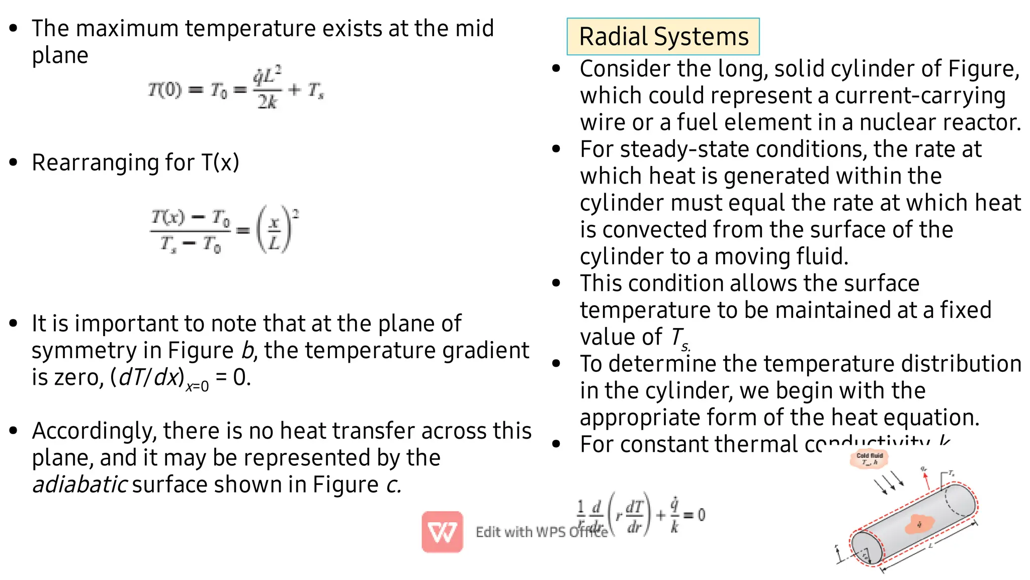
Consider the long, solid cylinder of Figure,
which could represent a current-carrying
wire or a fuel element in a nuclear reactor.
For steady-state conditions, the rate at
which heat is generated within the
cylinder must equal the rate at which heat
is convected from the surface of the
cylinder to a moving fluid.
This condition allows the surface
temperature to be maintained at a fixed
value of Ts.
To determine the temperature distribution
in the cylinder, we begin with the
appropriate form of the heat equation.
For constant thermal conductivity k,
Radial Systems

23. •
•
•
•
Separating variables and assuming uniform
generation, this expression may be integrated
to obtain
Repeating the procedure, the general solution
for the temperature distribution becomes
To obtain the constants of integration C1 and C2,
we apply the boundary conditions
The temperature distribution is therefore
• We obtain the temperature distribution in
non-dimensional form,
•
•
•
where To is the centerline temperature.
The heat rate at any radius in the cylinder may,
of course, be evaluated by using Fourier’s law.
To relate the surface temperature, Ts, to the
temperature of the cold fluid T
, either a
surface energy balance or an overall energy
balance may be used.
Choosing the second approach, we obtain

24. Heat
Transfer
from
Extended
Surfaces
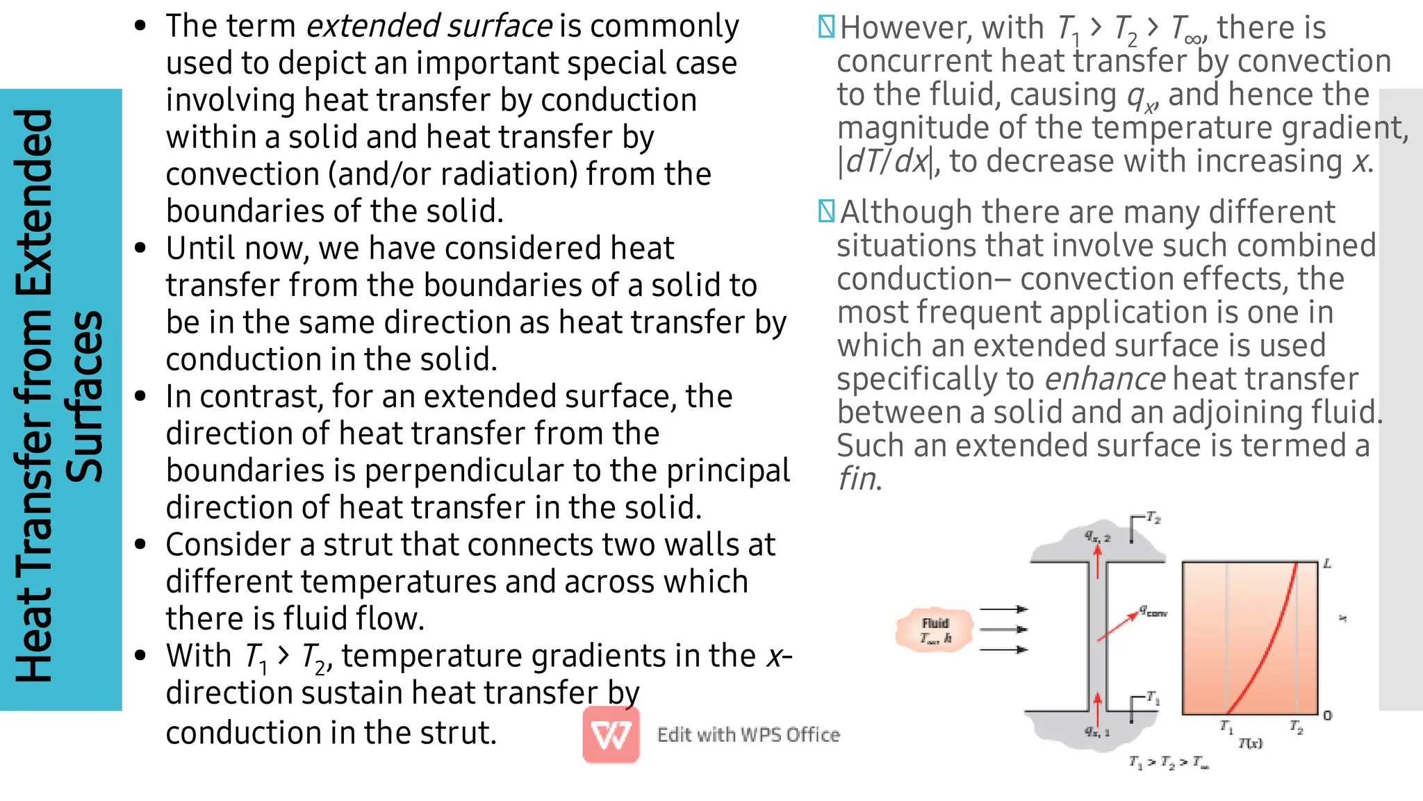
However, with T1 > T2 > T∞, there is
concurrent heat transfer by convection
to the fluid, causing qx, and hence the
magnitude of the temperature gradient,
|dT/dx|, to decrease with increasing x.
Although there are many different
situations that involve such combined
conduction– convection effects, the
most frequent application is one in
which an extended surface is used
specifically to enhance heat transfer
between a solid and an adjoining fluid.
Such an extended surface is termed a
fin.
•
•
•
•
•
The term extended surface is commonly
used to depict an important special case
involving heat transfer by conduction
within a solid and heat transfer by
convection (and/or radiation) from the
boundaries of the solid.
Until now, we have considered heat
transfer from the boundaries of a solid to
be in the same direction as heat transfer by
conduction in the solid.
In contrast, for an extended surface, the
direction of heat transfer from the
boundaries is perpendicular to the principal
direction of heat transfer in the solid.
Consider a strut that connects two walls at
different temperatures and across which
there is fluid flow.
With T1 > T2, temperature gradients in the x-
direction sustain heat transfer by
conduction in the strut.

25. •
•
•
•
•
•
•
•
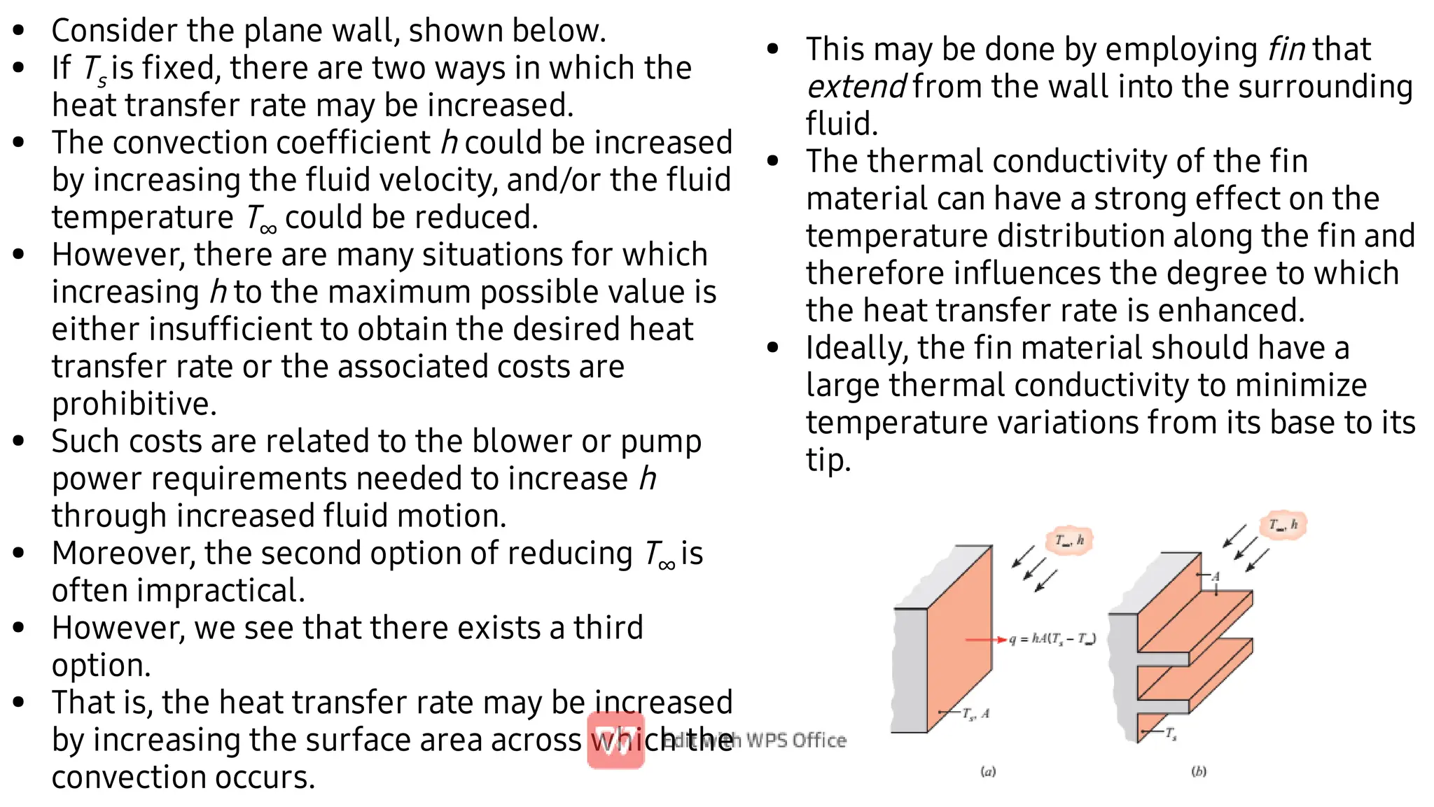
Consider the plane wall, shown below.
If Ts is fixed, there are two ways in which the
heat transfer rate may be increased.
The convection coefficient h could be increased
by increasing the fluid velocity, and/or the fluid
temperature T∞ could be reduced.
However, there are many situations for which
increasing h to the maximum possible value is
either insufficient to obtain the desired heat
transfer rate or the associated costs are
prohibitive.
Such costs are related to the blower or pump
power requirements needed to increase h
through increased fluid motion.
Moreover, the second option of reducing T∞ is
often impractical.
However, we see that there exists a third
option.
That is, the heat transfer rate may be increased
by increasing the surface area across which the
convection occurs.
•
•
•
This may be done by employing fin that
extend from the wall into the surrounding
fluid.
The thermal conductivity of the fin
material can have a strong effect on the
temperature distribution along the fin and
therefore influences the degree to which
the heat transfer rate is enhanced.
Ideally, the fin material should have a
large thermal conductivity to minimize
temperature variations from its base to its
tip.

26. •
•
•
In the limit of infinite thermal conductivity, the
entire fin would be at the temperature of the
base surface, thereby providing the maximum
possible heat transfer enhancement.
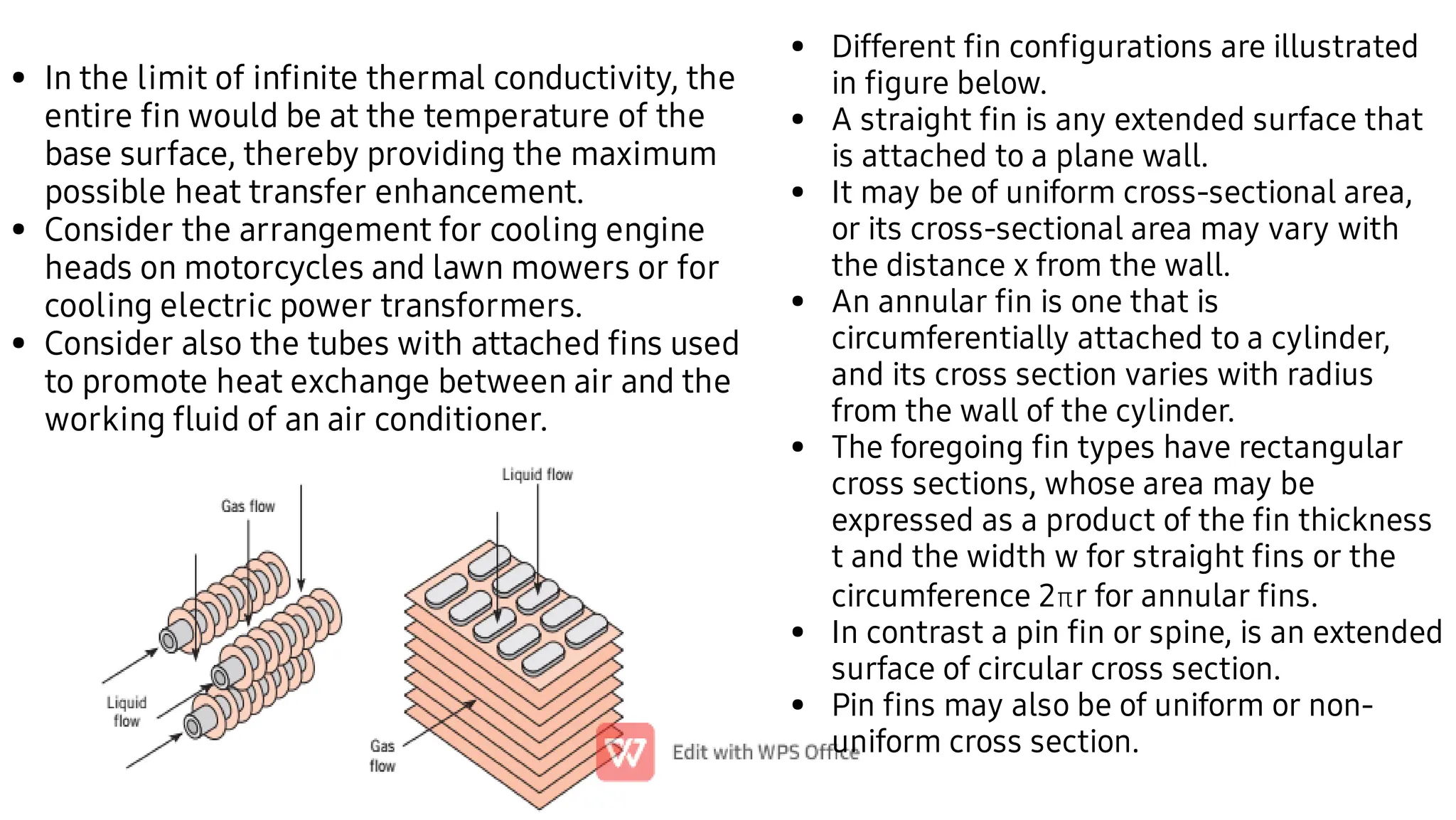
Consider the arrangement for cooling engine
heads on motorcycles and lawn mowers or for
cooling electric power transformers.
Consider also the tubes with attached fins used
to promote heat exchange between air and the
working fluid of an air conditioner.
•
•
•
•
•
•
•
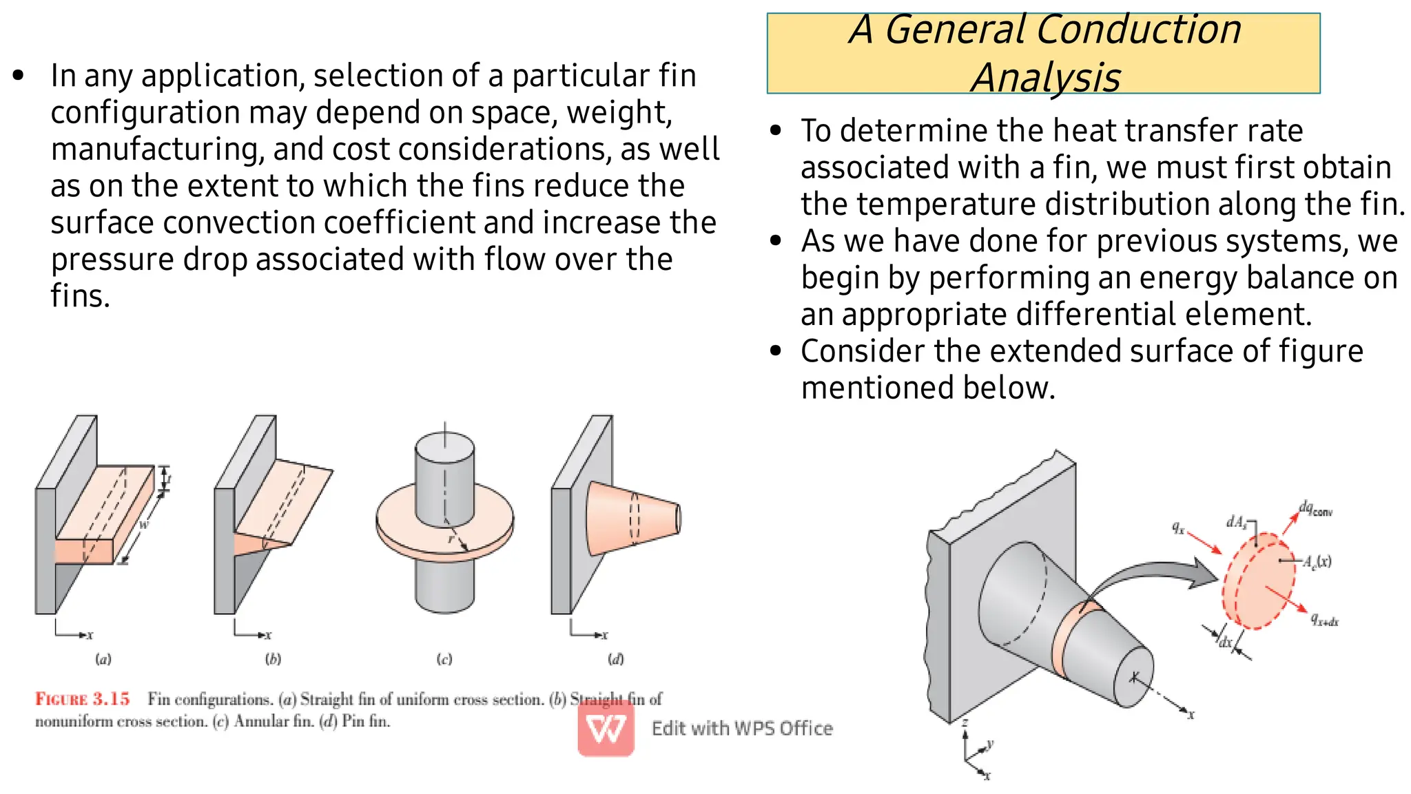
Different fin configurations are illustrated
in figure below.
A straight fin is any extended surface that
is attached to a plane wall.
It may be of uniform cross-sectional area,
or its cross-sectional area may vary with
the distance x from the wall.
An annular fin is one that is
circumferentially attached to a cylinder,
and its cross section varies with radius
from the wall of the cylinder.
The foregoing fin types have rectangular
cross sections, whose area may be
expressed as a product of the fin thickness
t and the width w for straight fins or the
circumference 2r for annular fins.
In contrast a pin fin or spine, is an extended
surface of circular cross section.
Pin fins may also be of uniform or non-
uniform cross section.

27. • In any application, selection of a particular fin
configuration may depend on space, weight,
manufacturing, and cost considerations, as well
as on the extent to which the fins reduce the
surface convection coefficient and increase the
pressure drop associated with flow over the
fins.
•
•
•
To determine the heat transfer rate
associated with a fin, we must first obtain
the temperature distribution along the fin.
As we have done for previous systems, we
begin by performing an energy balance on
an appropriate differential element.
Consider the extended surface of figure
mentioned below.
A General Conduction
Analysis

28. •
•
•
•
•
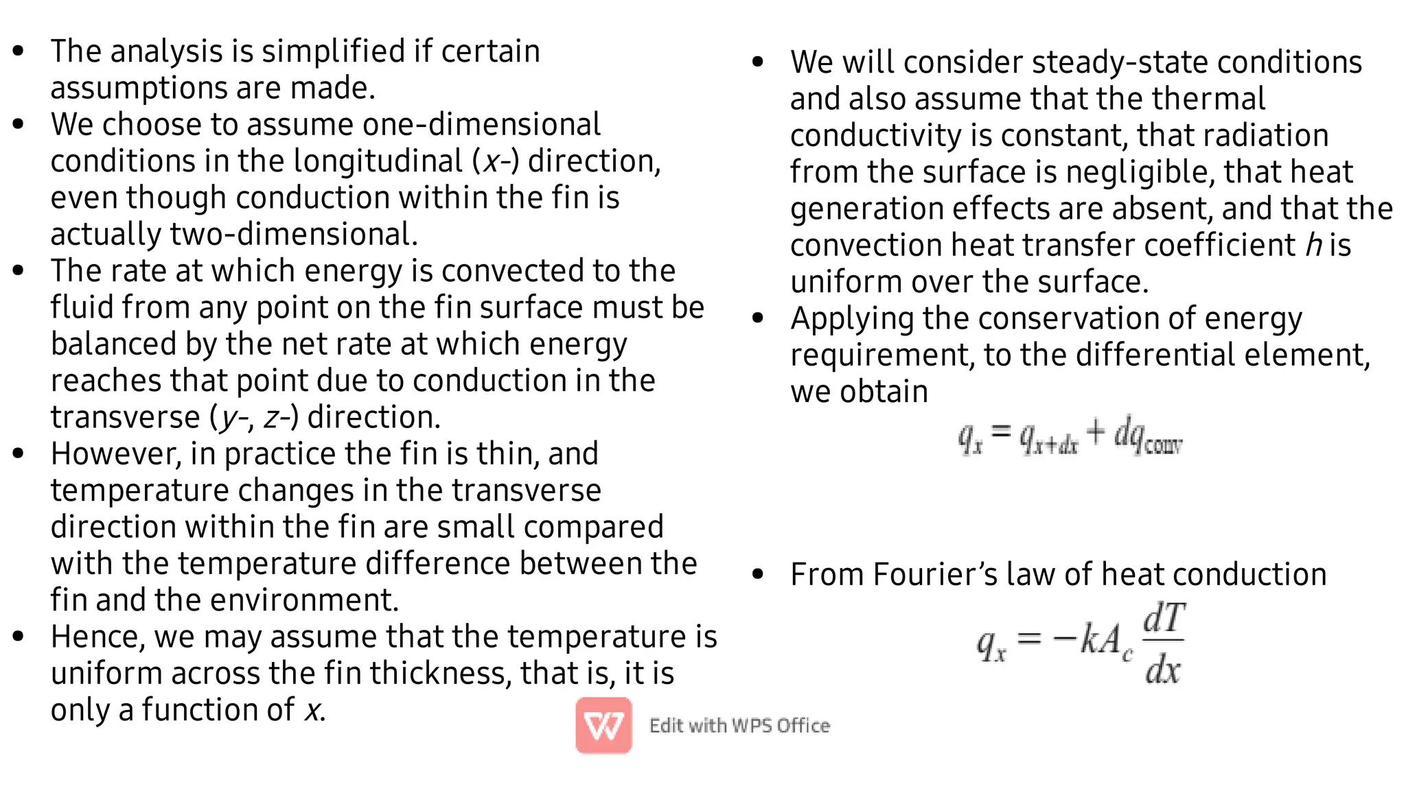
The analysis is simplified if certain
assumptions are made.
We choose to assume one-dimensional
conditions in the longitudinal (x-) direction,
even though conduction within the fin is
actually two-dimensional.
The rate at which energy is convected to the
fluid from any point on the fin surface must be
balanced by the net rate at which energy
reaches that point due to conduction in the
transverse (y-, z-) direction.
However, in practice the fin is thin, and
temperature changes in the transverse
direction within the fin are small compared
with the temperature difference between the
fin and the environment.
Hence, we may assume that the temperature is
uniform across the fin thickness, that is, it is
only a function of x.
•
•
•
We will consider steady-state conditions
and also assume that the thermal
conductivity is constant, that radiation
from the surface is negligible, that heat
generation effects are absent, and that the
convection heat transfer coefficient h is
uniform over the surface.
Applying the conservation of energy
requirement, to the differential element,
we obtain
From Fourier’s law of heat conduction

29. •
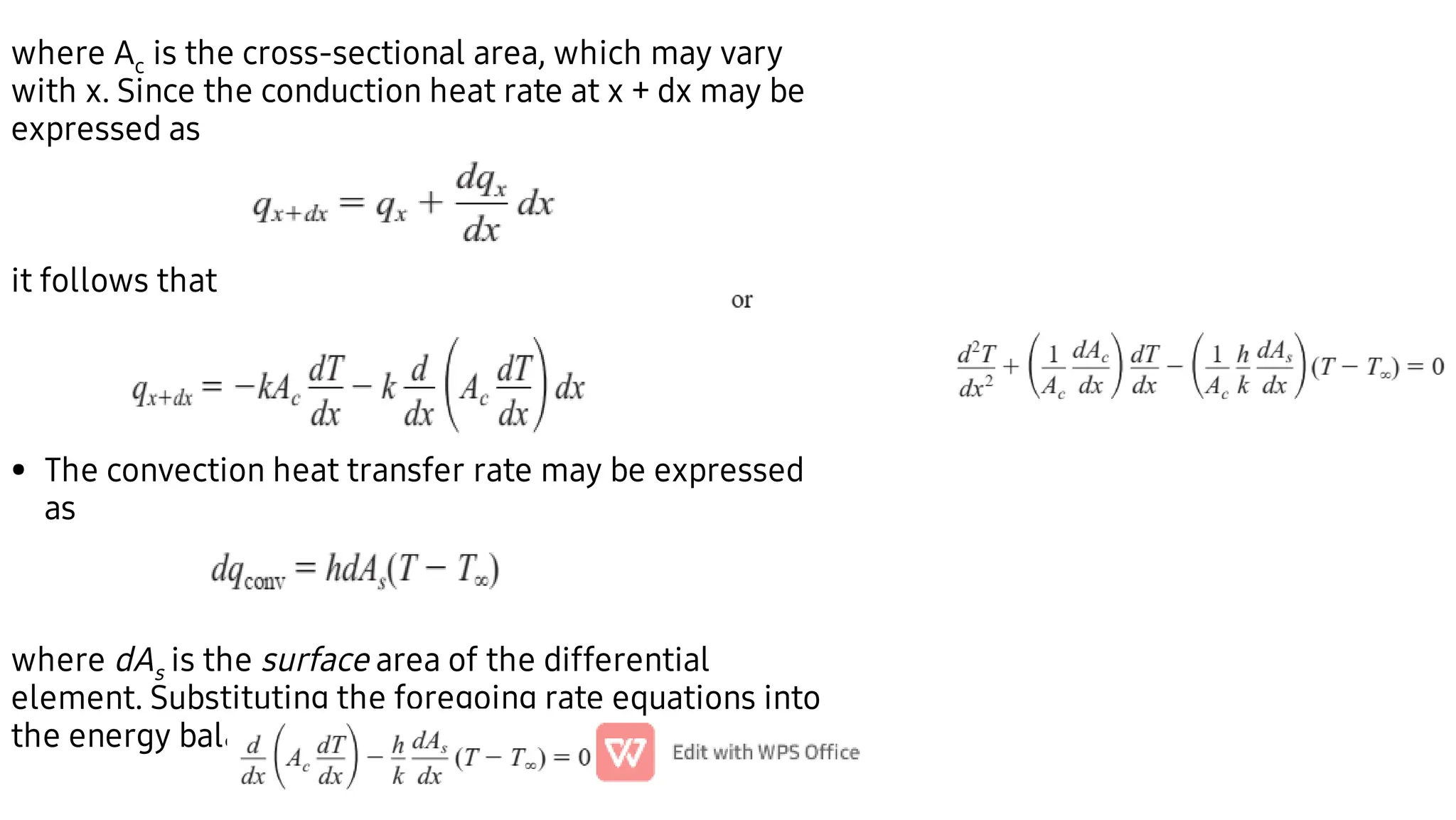
where Ac is the cross-sectional area, which may vary
with x. Since the conduction heat rate at x + dx may be
expressed as
it follows that
The convection heat transfer rate may be expressed
as
where dAs is the surface area of the differential
element. Substituting the foregoing rate equations into
the energy balance

30. Fins
of
Uniform
Cross-
Sectional
Area
•
•
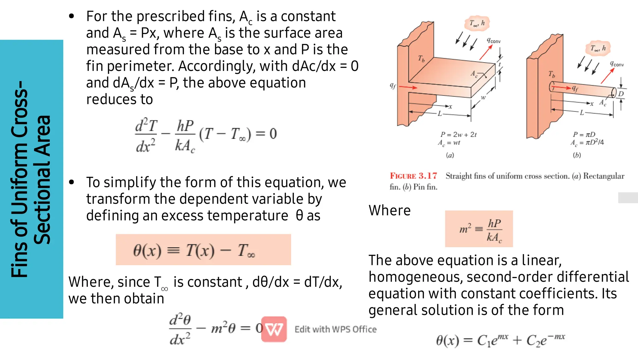
For the prescribed fins, Ac is a constant
and As = Px, where As is the surface area
measured from the base to x and P is the
fin perimeter. Accordingly, with dAc/dx = 0
and dAs/dx = P, the above equation
reduces to
To simplify the form of this equation, we
transform the dependent variable by
defining an excess temperature θ as
Where, since T is constant , dθ/dx = dT/dx,
we then obtain
Where
The above equation is a linear,
homogeneous, second-order differential
equation with constant coefficients. Its
general solution is of the form

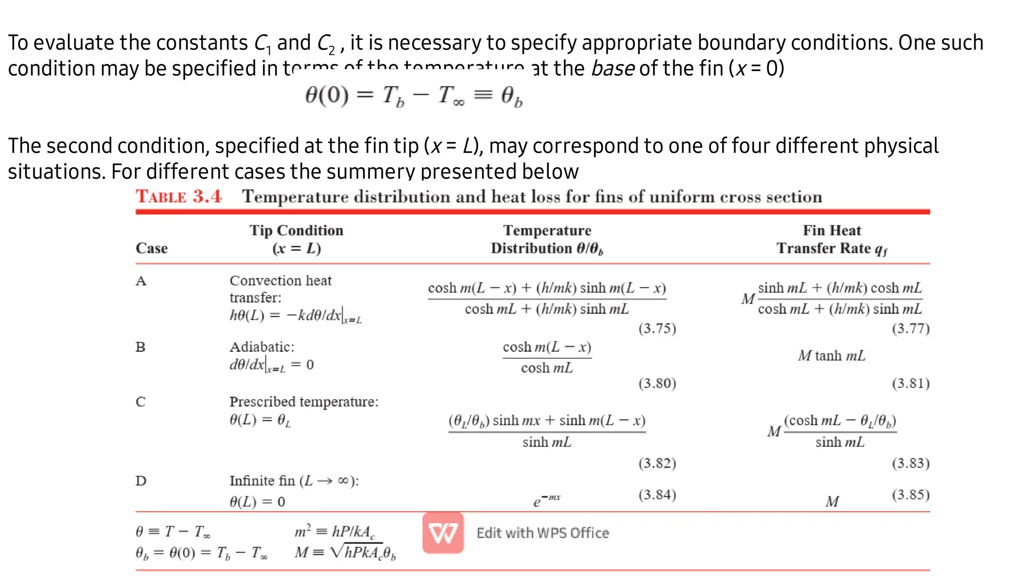
31. To evaluate the constants C1 and C2 , it is necessary to specify appropriate boundary conditions. One such
condition may be specified in terms of the temperature at the base of the fin (x = 0)
The second condition, specified at the fin tip (x = L), may correspond to one of four different physical
situations. For different cases the summery presented below