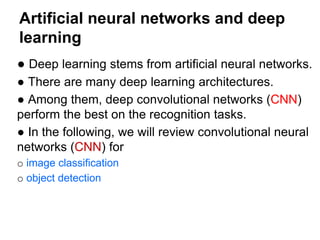
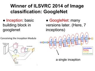
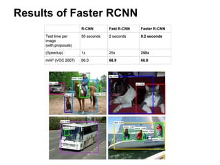
This document discusses deep learning techniques for object detection and recognition. It provides an overview of computer vision tasks like image classification and object detection. It then discusses how crowdsourcing large datasets from the internet and advances in machine learning, specifically deep convolutional neural networks (CNNs), have led to major breakthroughs in object detection. Several state-of-the-art CNN models for object detection are described, including R-CNN, Fast R-CNN, Faster R-CNN, SSD, and YOLO. The document also provides examples of applying these techniques to tasks like face detection and detecting manta rays from aerial videos.

1. Deep Learning Techniques for
Object Detection and Recognition
Chu-Song Chen

2. Outline
● Computer Vision
● Image Classification and Object Detection
● Crowdsourcing + Machine Learning
o Image Net + ILSVRC Challenge
o Deep Convolution Nets
● Recent Advances and Results

3. Computer Vision
● Research on the methods for acquiring, processing,
analyzing, and understanding images and, in general, high-
dimensional data from the real world in order to produce
numerical or symbolic information, e.g., in the forms of
decisions.

4. Object Detection & Recognition
● Object recognition is one of the main tasks in
computer vision.
Semantic segmentation Object detection

5. What is object detection?
● Image classification
● object localization
● object detection
● segmentation
difficulty

6. Why is object detection important?
● Perception is one of the biggest bottlenecks of
○ Robotics
○ Self-driving cars
○ Surveillance

7. Applications
● Image classification
○ image search (Google, Baidu, Bing)
● Object detection
○ face
■ smart phone/cameras
■ election duplicate votes
■ CCTV
■ border control
■ casinos
■ visa processing
■ crime solving
■ prosopagnosia (face blindness)
○ objects
■ license plates
■ pedestrian detection (Daimler, MobileEye):
● warning and automatic braking reducing accidents
and severity
■ vehicle detection for forward collision
warning (MobileEye)
■ traffic sign detection (MobileEye)
 E-commerce
 machine inspection

8. Machine Learning & Computer
Vision
● How to achieve object recognition?
o Typically through machine learning in computer vision.
● Training stage:
o Collect training sample images.
o Learn an object detector.
● Inference stage: Employ the learned detector for detection.
o Take pedestrian detection as an example:

9. Pedestrian detection: training phase
(traditional approach)
● Collecting training data
o Extracting features (or casting data into feature space).
 color, edge, gradient, silhouette, dimension reduction, etc.
o Learning an object detector classifier
 Many learning methods: eg., Neural Networks, SVM,
Boosting, Cascaded AdaBoost, random forest.
Positive training data Negative training data

10. 10
Pedestrian detection: testing phase
(traditional approach)
● After learning a human detector
o A detection window can be used to scan the testing image
along x and y directions for human detection.

11. 11
Pedestrian detection: inference phase
● Human detection
o Detection windows with different sizes are used to detect
humans with different scales.
…
…
…

12. Difficulties for object recognition
● Object recognition
To human (an image and an image block)
To machine (a data ary of real numbers)

13. Past breakthroughs in object
detection researches
o Face detection: Haar
feature + AdaBoost
learning. (2000)
● Every mobile phone is
equipped with this function now.
o SIFT and HOG: local
discriminating features.
(2004) + SVM for object
detection.
● A key component to RGB vision-
based positioning and localization.

14. Examples of several breakthroughs
in object detection researches
● Deformable part models (2008):
o HOG feature
o Latent SVM + stochastic gradient descent (SGD) training
o Training scale of the above: 5K ~ 20K training images.

15. General object recognition
o The above methods bring many ingredient in application.
o However, they are still difficult to achieve general object
detection/recognition.
● Recent big breakthroughs of object detection
comes from crowdsourcing + machine learning:
o More labeled training data are gathered from mechanical
turk.
o More suitable machine learning techniques: deep
convolution neural networks (CNNs).

16. Artificial neural networks and deep
learning
● Why deep learning?
o A limitation of tradition methods: separate feature
extraction and classifier training as two independent
processes.
o One motivation in deep learning is to joining feature
extraction and classification into a single framework.
o This causes a large number of parameters. However,
when the number of training images is huge, the issue of
over-fitting is lessened.
o Deep learning: end-to-end learning.
That is feature extraction + classification in a single step

17. slide: R. Fergus

18. slide: R. Fergus

21. slide: Honglak Lee

22. Artificial neural networks and deep
learning
● Deep learning stems from artificial neural networks.
● There are many deep learning architectures.
● Among them, deep convolutional networks (CNN)
perform the best on the recognition tasks.
● In the following, we will review convolutional neural
networks (CNN) for
o image classification
o object detection

23. Convoltional Neural Networks
● CNN: a neural network consists of
o fully-connected layer
o convolution layer
o max-pooling
o nonlinear activation (ReLU or sigmoid)
o ………

24. Fully-connected layers
● If the input is an image, the fully connected layer
will have a huge amount of links between layers:
● The weights are required to be learned.

25. Convolution layer
● Instead of fully connection, using a 𝑘𝑘 × 𝑘𝑘 widow to slide the
image and performing inner product on every site.
● That is, applying a 𝑘𝑘 × 𝑘𝑘 FIR filter or convolution on the image.
● The coefficients are required to be learned.

26. Convolution vs. fully-connection
●.Convolutional layer:
o Shared weights
o Shift invariance
o Local
Convolutional layer Fully connected layer

27. Multiple FIR filters in a convolutional layer
● Often multiple FIR filters are in a convolutional layer.
● The filters’ outputs serves the inputs of the next layer.
● So, if the number of filters used in a convolution layer
are a number of 𝑐𝑐𝑙𝑙, the output of this layer forms an 𝑛𝑛𝑙𝑙 ×
𝑛𝑛𝑙𝑙 × 𝑐𝑐𝑙𝑙 volume.
𝑛𝑛𝑙𝑙
𝑛𝑛𝑙𝑙

28. Multiple “volume” FIR filters
● So, the output of the convolution layer has 𝑐𝑐𝑙𝑙
channels, forming an 𝑛𝑛𝑙𝑙 × 𝑛𝑛𝑙𝑙 × 𝑐𝑐𝑙𝑙 volume.
● Actually, the FIR filters applied in a CNN are
of size 𝑘𝑘 × 𝑘𝑘 × 𝑐𝑐𝑙𝑙 (though we usually
abbreviate it as 𝑘𝑘 × 𝑘𝑘 in for simplicity); it is
indeed a “volume” FIR filter).

29. Input: a RGB (3-chanel) image of size 𝑁𝑁 × 𝑁𝑁
● Eg., 𝑁𝑁 = 32, input to the first convolutional layer having 5
filters
● Eg., 𝑁𝑁 = 40, input to a cascade of convolutional layers, a
fully connected layer, and the final output layer. (entire network)

30. A single
neuron
o activation
function example
o sigmoid
o ReLU
z
Nonlinear activation function
● or if the layers are cascaded linearly, they can be replaced
by a single equivalent layer.

31. Pooling for dimension (size)
reduction
or the weights will still be.
 Summaries the input
● Eg, Max pooling

32. Max pooling layer (cont)
After max
pooling, the size
(i.e., dimension)
of the feature
map is reduced.

33. ● Sharing parameters is good
○ taking advantage of local coherence to learn a more efficient representation:
■ no redundancy
■ translation invariance
■ slight rotation invariance with pooling
● Efficient for detection:
○ all computations are shared
○ can handle varying input sizes (no need to relearn weights for new sizes)
● ConvNets are convolutional all the way up including fully connected layers
Why are ConvNets good for detection?
slide: Pierre Sermanett

34. Big-data training images from Internet
● ILSVRC competition (ImageNet Challenge)
o ImageNet: collecting images according to the Wordnet tree.
o ILSVRC: choosing words in different tree branches.

35. ILSVRC Image classification
challenge

36. Fine tuning
● ILSVRC (ImageNet challenge) is a large
dataset with diverse object classes.
● Using the pre-trained weights on ILSVRC for
fine-tuning is a popular strategy.

37. Winner of ILSVRC 2012 of Image
classification: AlexNet
• 5 convolutional layers, 3 fully-connected layers
• The number of neurons in each layer is given by 253440, 186624, 64896, 64896, 43264,
4096, 4096, 1000.
● This was made possible by:
○ fast hardware: GPU-optimized code
○ big dataset: 1.2 million images vs thousands before
○ better regularization: dropout

38. Winner of ILSVRC 2014 of Image
classification: GoogleNet
● Inception: basic
building block in
googlenet
● GoogleNet: many
versions later. (Here, 7
inceptions)
a single inception

39. ILSVRC 2014 Single-net best performed –
VGG network (11- 19 layers)
Design criterion:
Using 3 × 3 filters
(to find small
details in every
layer)
Max-pooling (half-
size reduced of
the height and
width of the
feature map)
+
Double the
number of feature
maps by doubling
the filters.

40. ILSVRC 2015 winner – Residual
network (50- 151 layers)
Design criterion:
Add the short-cut link
Fully connected layer → average
pooling
Use batch normalization

41. From image classification to object
detection
● The above CNNs are designed for image classification (i.e.,
assume only one concept is contained in the input image).
● However, they serve as important building blocks for
feature extraction, and can be migrated to a new architecture
for object detection.
Image classification task
Object detection task

42. Object detection CNNs
● RCNN – Fast RCNN – Raster RCNN
● RFCN
● SSD
● PVA net
● Yolo v2
● ……

43. R-CNN
●R-CNN: Regions with CNN features
43
Koen E. A. van de Sande, Jasper R. R.
Uijlings, Theo Gevers, Arnold W. M. Smeulders,
Segmentation As Selective Search for
Object Recognition, in ICCV 2011

44. ● Scan the input image for possible objects using an algorithm called Selective
Search, generating ~2000 region proposals
● Run a convolutional neural net (CNN) on top of each of these region proposals.
The CNN are pre-trained on the ImageNet and fine-tuned here.
● Take the output of each CNN and feed it into a) an SVM to classify the region
and b) a regressor to tighten the bounding box of the object, if such an object
exists.

45. ● bounding box regression: output the center
and size of tight bounding box of the object.

46. ● Generate region proposals based on the last feature map of the network, not from the
original image itself. As a result, we can train just one CNN for the entire image.
● The CNN is fined-tuned from the image classification network pre-trained on ImageNet.
● However, selective search in the original image is still needed.
● Without using SVMs: replacing SVMs with the CNN output.

47. ● At the last layer of an initial CNN, a 3x3 sliding window moves across the feature map
and maps it to a lower dimension (e.g. 256-d)
● For each sliding-window location, it generates multiple possible regions based on k
fixed-ratio anchor boxes (default bounding boxes)
● Each region proposal consists of a) an “objectness” score for that region and b) 4
coordinates representing the bounding box of the region
Faster RCNN: region proposal ntwork

48. ● The main insight of Faster R-CNN was to replace the slow selective search algorithm
with a fast neural net. Specifically, it introduced the region proposal network (RPN).
● Faster R-CNN = RPN + Fast R-CNN

49. ● In other words, look at each location in our last feature map and consider 𝑘𝑘 boxes
centered around it: a tall, a wide, and a large box, etc. For each of those boxes, output
whether or not we think it contains an object, and what the coordinates for that box are.
● Feed the proposal into what is essentially a Fast R-CNN.
● Union the CNN in the bottom for both the region proposal network in faster RCNN and
the bounding-box-regression/object-classification in fast RCNN.

50. Results of Faster RCNN

51. SSD
● Region proposal and classification are trained simultaneously, unlike faster
RCNN that they are trained alternatively.
● Early convolution layers are also used. Early layers corresponds to smaller
objects, and rear layers corresponds to large objects.
● Faster and performance even better than faster RCNN

52. Yolo v2 (cvpr 2017)
● Modified from faster RCNN and Yolo
o use batch normalization; remove dropout.
o higher-resolution CNN classifier pretrained: from 224 ×
224 to 448 × 448
o use 9000 classes in the ImageNet for pre-training, instead
of 1000.
o direct location prediction: solve the instability in the
bounding box regression of faster RCNN.
● state-of-the-art on standard detection tasks like PASCAL
VOC and COCO datasets.
o At 67 FPS, YOLOv2 gets 76.8 mAP on VOC 2007. At 40 FPS, YOLOv2 gets
78.6 mAP, outperforming state-of-the-art methods like Faster RCNN with ResNet
and SSD while still running significantly faster.

53. Dataset
●Total 9,667 images:
o1,964 images annotated by ourselves
o7,703 images with bounding annotations from a public
dataset (ATR)
53
Applications: faster RCNN for clothing
detection

54. Dataset (Cont’d)
●9 categories:
●bag, belt, dress, footwear, glasses, hat, pants, skirt,
upperclothes
●# bounding boxes per category
54

55. LabelMe Annotation Tool
● A web-based tool to
create bounding boxes
and assign labels.
55

56. 56
Ournotated
dataATR

57. Detection Results
57
Approach: Faster RCNN

58. Quantitative Results
● Metric: mAP (mean Average Precision)
● A detection is considered correct if its IoU
(intersection over union) with ground truth ≥
0.5 and its label is correct.
●Detection performance
58

59. Quantitative Results
●Metric: mAP (mean Average Precision)
●A detection is considered correct if its IoU
(Intersection over union) with ground truth ≥
0.5 and its label is correct.
●Detection performance
59
❏Perform better on larger items, e.g., upperclothes, dress, pants

60. Quantitative Results
●Metric: mAP (mean Average Precision)
●A detection is considered correct if its IoU
(Intersection over union) with ground truth ≥
0.5 and its label is correct.
●Detection performance
60
❏Perform better on larger items, e.g., upperclothes, dress, pants
❏Belts are very difficult to detect.

61. Summary
● The clothes item detector trained with
bounding box annotations can produce
satisfactory results. Even only a small set of
training data is applied.
● Trainin data is an issue: It is time-consuming
to obtain ground-truth bounding boxes.
61

62. Face detection
● Face-detection CNN: it is trained on a large-
scale face image dataset following similar ideas.
● We show that the face detector can be
realized in a CPU-based machine, Zenbo.

63. Deep CNN face detection/alignment
on Zenbo
●Zenbo Specifications
o CPU: Intel Atom x5-Z8550 2.4 GHz
o OS: Android 6.0.1
o RAM: 4G
o without using GPUs
● Frames per second
o 2.5 FPS [Resolution (640x480) ]
● Code optimizations
o C++ and OpenBLAS library
o Multi-threads computation
o without using any deep learning frameworks such as
tensorflow or pytorch

64. 海洋空拍機魟魚偵測
● Chien-Hung Chen’s master thesis (Dept. of
Mech. & Elec. Mach. Eng., NSYSU)；
● advisor: Prof. Keng-Hao Liu
A difficult problem: human may fail to track all
the 魟魚 successfully.
● Using Faster RCNN to train and detect
 base net: ZF or VGG
 Detection based on a video; using continuous
frames to refine the results.

65. Demo (close range)
ZF model VGG model
ZF model with time information VGG model with time information

66. Demo (distant range)
ZF model VGG model
ZF model with time information VGG model with time information

67. Demo (hard case)
ZF model VGG model
ZF model with time information VGG model with time information

68. Quantitative Results
● In the ground-truth, some 魟魚 sequences
detected by our method are not marked by human.
● After re-investigating these cases with human
experts, they have re-marked them as ground
truth.
Results of some video

69. Applicatins of deep CNN detector
● Deep CNN object detection techniques have
grown very fast in recent years. Several
promising models have been developed.
● The methods can be used for machine
inspection.
● Preparing data (with ground-truth regions)
would be an issue.
o Make the data type diverse
o If only few data with labeled regions can be collected,
augmenting the data by some attack (eg., by flipping,
rotation, cropping, lighting changes, blurring, sharpening
JPEG, etc.) is a useful technique for training.

70. Acknowledgement
Part of the slides are from the tutorial of CVPR2014, Deep
Learning for Computer Vision.