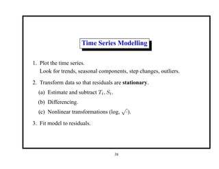
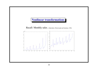
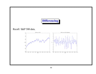
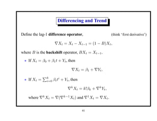
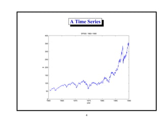
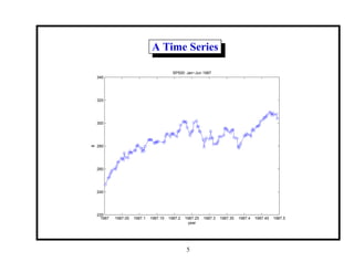
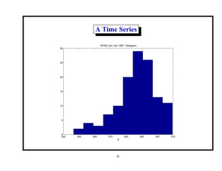
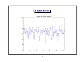
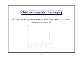
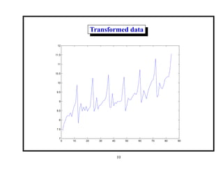
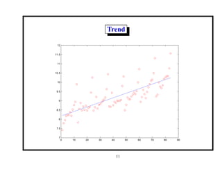
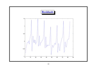
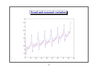
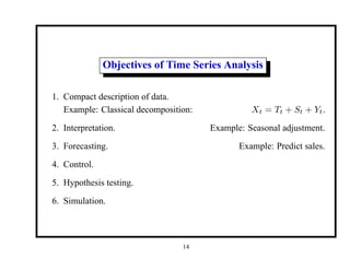
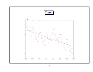
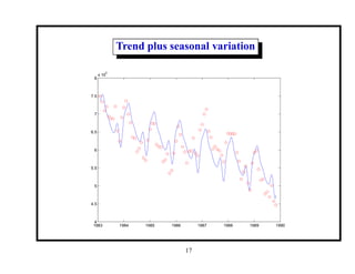
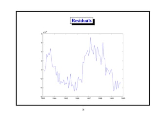
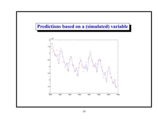
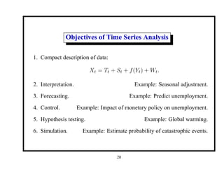
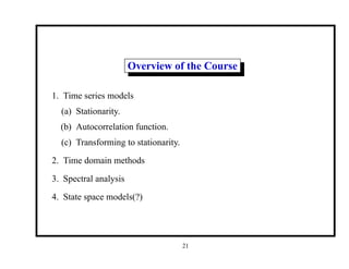
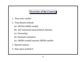
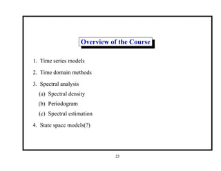
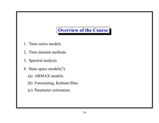
This document provides an introduction and overview of a time series analysis course. It discusses the objectives of time series analysis including compact description of data, interpretation, forecasting, control, hypothesis testing and simulation. Examples of decomposing time series into trend, seasonal and residual components are presented. The course will cover time series models, time domain methods like ARMA modeling, spectral analysis, and state space models. Stationarity, autocorrelation, differencing, and nonlinear transformations are discussed as ways to make time series stationary.

1. Introduction to Time Series Analysis. Lecture 1.
Peter Bartlett
1. Organizational issues.
2. Objectives of time series analysis. Examples.
3. Overview of the course.
4. Time series models.
5. Time series modelling: Chasing stationarity.
1

2. Organizational Issues
• Peter Bartlett. bartlett@stat. Office hours: Thu 1:30-2:30 (Evans 399).
Fri 3-4 (Soda 527).
• Brad Luen. bradluen@stat. Office hours: Tue/Wed 2-3pm (Room
TBA).
• http://www.stat.berkeley.edu/∼bartlett/courses/153-fall2005/
Check it for announcements, assignments, slides, ...
• Text: Time Series Analysis and its Applications, Shumway and Stoffer.
2

3. Organizational Issues
Computer Labs: Wed 12–1 and Wed 2–3, in 342 Evans.
You need to choose one of these times. Please email bradluen@stat with
your preference. First computer lab sections are on September 7.
Classroom Lab Section: Fri 12–1, in 330 Evans. First classroom lab
section is on September 2.
Assessment:
Lab/Homework Assignments (40%): posted on the website.
These involve a mix of pen-and-paper and computer exercises. You may use
any programming language you choose (R, Splus, Matlab). The last
assignment will involve analysis of a data set that you choose.
Midterm Exam (25%): scheduled for October 20, at the lecture.
Final Exam (35%): scheduled for Thursday, December 15.
3

4. A Time Series
1960 1965 1970 1975 1980 1985 1990
0
50
100
150
200
250
300
350
400
year
$
SP500: 1960−1990
4

5. A Time Series
1987 1987.05 1987.1 1987.15 1987.2 1987.25 1987.3 1987.35 1987.4 1987.45 1987.5
220
240
260
280
300
320
340
year
$
SP500: Jan−Jun 1987
5

6. A Time Series
240 250 260 270 280 290 300 310
0
5
10
15
20
25
30
$
SP500 Jan−Jun 1987. Histogram
6

7. A Time Series
0 20 40 60 80 100 120
220
240
260
280
300
320
340
$
SP500: Jan−Jun 1987. Permuted.
7

8. Objectives of Time Series Analysis
1. Compact description of data.
2. Interpretation.
3. Forecasting.
4. Control.
5. Hypothesis testing.
6. Simulation.
8

9. Classical decomposition: An example
Monthly sales for a souvenir shop at a beach resort town in Queensland.
(Makridakis, Wheelwright and Hyndman, 1998)
0 10 20 30 40 50 60 70 80 90
0
2
4
6
8
10
12
x 10
4
9

10. Transformed data
0 10 20 30 40 50 60 70 80 90
7
7.5
8
8.5
9
9.5
10
10.5
11
11.5
12
10

11. Trend
0 10 20 30 40 50 60 70 80 90
7
7.5
8
8.5
9
9.5
10
10.5
11
11.5
12
11

12. Residuals
0 10 20 30 40 50 60 70 80 90
−1
−0.5
0
0.5
1
1.5
12

13. Trend and seasonal variation
0 10 20 30 40 50 60 70 80 90
7
7.5
8
8.5
9
9.5
10
10.5
11
11.5
12
13

14. Objectives of Time Series Analysis
1. Compact description of data.
Example: Classical decomposition: Xt = Tt + St + Yt.
2. Interpretation. Example: Seasonal adjustment.
3. Forecasting. Example: Predict sales.
4. Control.
5. Hypothesis testing.
6. Simulation.
14

15. Unemployment data
Monthly number of unemployed people in Australia. (Hipel and McLeod, 1994)
1983 1984 1985 1986 1987 1988 1989 1990
4
4.5
5
5.5
6
6.5
7
7.5
8
x 10
5
15

16. Trend
1983 1984 1985 1986 1987 1988 1989 1990
4
4.5
5
5.5
6
6.5
7
7.5
8
x 10
5
16

17. Trend plus seasonal variation
1983 1984 1985 1986 1987 1988 1989 1990
4
4.5
5
5.5
6
6.5
7
7.5
8
x 10
5
17

18. Residuals
1983 1984 1985 1986 1987 1988 1989 1990
−6
−4
−2
0
2
4
6
8
x 10
4
18

19. Predictions based on a (simulated) variable
1983 1984 1985 1986 1987 1988 1989 1990
4
4.5
5
5.5
6
6.5
7
7.5
8
x 10
5
19

20. Objectives of Time Series Analysis
1. Compact description of data:
Xt = Tt + St + f(Yt) + Wt.
2. Interpretation. Example: Seasonal adjustment.
3. Forecasting. Example: Predict unemployment.
4. Control. Example: Impact of monetary policy on unemployment.
5. Hypothesis testing. Example: Global warming.
6. Simulation. Example: Estimate probability of catastrophic events.
20

21. Overview of the Course
1. Time series models
(a) Stationarity.
(b) Autocorrelation function.
(c) Transforming to stationarity.
2. Time domain methods
3. Spectral analysis
4. State space models(?)
21

22. Overview of the Course
1. Time series models
2. Time domain methods
(a) AR/MA/ARMA models.
(b) ACF and partial autocorrelation function.
(c) Forecasting
(d) Parameter estimation
(e) ARIMA models/seasonal ARIMA models
3. Spectral analysis
4. State space models(?)
22

23. Overview of the Course
1. Time series models
2. Time domain methods
3. Spectral analysis
(a) Spectral density
(b) Periodogram
(c) Spectral estimation
4. State space models(?)
23

24. Overview of the Course
1. Time series models
2. Time domain methods
3. Spectral analysis
4. State space models(?)
(a) ARMAX models.
(b) Forecasting, Kalman filter.
(c) Parameter estimation.
24

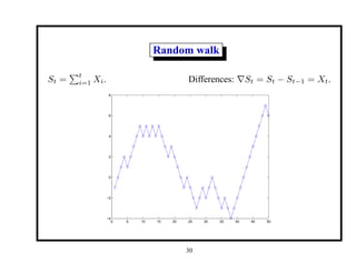
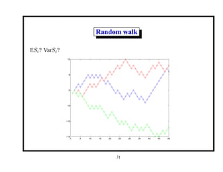
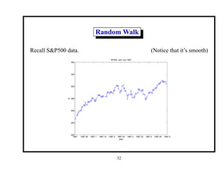
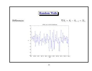
25. Time Series Models
A time series model specifies the joint distribution of the se-
quence {Xt} of random variables.
For example:
P[X1 ≤ x1, . . . , Xt ≤ xt] for all t and x1, . . . , xt.
Notation:
X1, X2, . . . is a stochastic process.
x1, x2, . . . is a single realization.
We’ll mostly restrict our attention to second-order properties only:
EXt, E(Xt1 Xt2 ).
25

26. Time Series Models
Example: White noise: Xt ∼ WN(0, σ2
).
i.e., {Xt} uncorrelated, EXt = 0, VarXt = σ2
.
Example: i.i.d. noise: {Xt} independent and identically distributed.
P[X1 ≤ x1, . . . , Xt ≤ xt] = P[X1 ≤ x1] · · · P[Xt ≤ xt].
Not interesting for forecasting:
P[Xt ≤ xt|X1, . . . , Xt−1] = P[Xt ≤ xt].
26

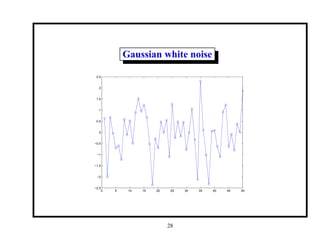
27. Gaussian white noise
P[Xt ≤ xt] = Φ(xt) =
1
√
2π
Z xt
−∞
e−x2
/2
dx.
0 5 10 15 20 25 30 35 40 45 50
−2.5
−2
−1.5
−1
−0.5
0
0.5
1
1.5
2
2.5
27

28. Gaussian white noise
0 5 10 15 20 25 30 35 40 45 50
−2.5
−2
−1.5
−1
−0.5
0
0.5
1
1.5
2
2.5
28

29. Time Series Models
Example: Binary i.i.d. P[Xt = 1] = P[Xt = −1] = 1/2.
0 5 10 15 20 25 30 35 40 45 50
−1
−0.8
−0.6
−0.4
−0.2
0
0.2
0.4
0.6
0.8
1
29

30. Random walk
St =
Pt
i=1 Xi. Differences: ∇St = St − St−1 = Xt.
0 5 10 15 20 25 30 35 40 45 50
−4
−2
0
2
4
6
8
30

31. Random walk
ESt? VarSt?
0 5 10 15 20 25 30 35 40 45 50
−15
−10
−5
0
5
10
31

32. Random Walk
Recall S&P500 data. (Notice that it’s smooth)
1987 1987.05 1987.1 1987.15 1987.2 1987.25 1987.3 1987.35 1987.4 1987.45 1987.5
220
240
260
280
300
320
340
year
$
SP500: Jan−Jun 1987
32

33. Random Walk
Differences: ∇St = St − St−1 = Xt.
1987 1987.05 1987.1 1987.15 1987.2 1987.25 1987.3 1987.35 1987.4 1987.45 1987.5
−10
−8
−6
−4
−2
0
2
4
6
8
10
year
$
SP500, Jan−Jun 1987. first differences
33

34. Trend and Seasonal Models
Xt = Tt + St + Et = β0 + β1t +
P
i (βi cos(λit) + γi sin(λit)) + Et
0 50 100 150 200 250
2.5
3
3.5
4
4.5
5
5.5
6
34

35. Trend and Seasonal Models
Xt = Tt + Et = β0 + β1t + Et
0 50 100 150 200 250
2.5
3
3.5
4
4.5
5
5.5
6
35

36. Trend and Seasonal Models
Xt = Tt + St + Et = β0 + β1t +
P
i (βi cos(λit) + γi sin(λit)) + Et
0 50 100 150 200 250
2.5
3
3.5
4
4.5
5
5.5
6
36

37. Trend and Seasonal Models: Residuals
0 50 100 150 200 250
−0.5
−0.4
−0.3
−0.2
−0.1
0
0.1
0.2
0.3
0.4
0.5
37

38. Time Series Modelling
1. Plot the time series.
Look for trends, seasonal components, step changes, outliers.
2. Transform data so that residuals are stationary.
(a) Estimate and subtract Tt, St.
(b) Differencing.
(c) Nonlinear transformations (log,
√
·).
3. Fit model to residuals.
38

39. Nonlinear transformations
Recall: Monthly sales. (Makridakis, Wheelwright and Hyndman, 1998)
0 10 20 30 40 50 60 70 80 90
0
2
4
6
8
10
12
x 10
4
0 10 20 30 40 50 60 70 80 90
7
7.5
8
8.5
9
9.5
10
10.5
11
11.5
12
39

40. Differencing
Recall: S&P 500 data.
1987 1987.05 1987.1 1987.15 1987.2 1987.25 1987.3 1987.35 1987.4 1987.45 1987.5
220
240
260
280
300
320
340
year
$
SP500: Jan−Jun 1987
1987 1987.05 1987.1 1987.15 1987.2 1987.25 1987.3 1987.35 1987.4 1987.45 1987.5
−10
−8
−6
−4
−2
0
2
4
6
8
10
year
$
SP500, Jan−Jun 1987. first differences
40

41. Differencing and Trend
Define the lag-1 difference operator, (think ‘first derivative’)
∇Xt = Xt − Xt−1 = (1 − B)Xt,
where B is the backshift operator, BXt = Xt−1.
• If Xt = β0 + β1t + Yt, then
∇Xt = β1 + ∇Yt.
• If Xt =
Pk
i=0 βiti
+ Yt, then
∇k
Xt = k!βk + ∇k
Yt,
where ∇k
Xt = ∇(∇k−1
Xt) and ∇1
Xt = ∇Xt.
41

42. Differencing and Seasonal Variation
Define the lag-s difference operator,
∇sXt = Xt − Xt−s = (1 − Bs
)Xt,
where Bs
is the backshift operator applied s times, Bs
Xt = B(Bs−1
Xt)
and B1
Xt = BXt.
If Xt = Tt + St + Yt, and St has period s (that is, St = St−s for all t), then
∇sXt = Tt − Tt−s + ∇sYt.
42

43. Least Squares Regression
Model: Xt = β0 + β1t + Wt
=
1 t


β0
β1

 + Wt,








X1
X2
.
.
.
XT








| {z }
x
=








1 1
1 2
.
.
.
.
.
.
1 T








| {z }
Z


β0
β1


| {z }
β
+








W1
W2
.
.
.
WT








| {z }
w
43

44. Least Squares Regression
x = Zβ + w.
Least squares: choose β to minimize kwk2
= kx − Zβk2
.
Solution β̂ satisfies the normal equations:
∇βkwk2
= 2Z0
(x − Zβ̂) = 0.
If Z0
Z is nonsingular, the solution is unique:
β̂ = (Z0
Z)−1
Z0
x.
44

45. Least Squares Regression
Properties of the least squares solution (β̂ = (Z0
Z)−1
Z0
x):
• Linear.
• Unbiased.
• For {Wt} i.i.d., it is the linear unbiased estimator with smallest
variance.
Other regressors Z: polynomial, trigonometric functions, piecewise
polynomial (splines), etc.
45

46. Outline
1. Objectives of time series analysis. Examples.
2. Overview of the course.
3. Time series models.
4. Time series modelling: Chasing stationarity.
46