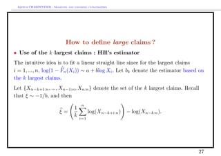
Download as PDF, PPTX

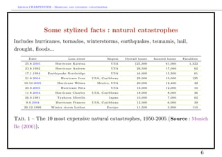

![Arthur CHARPENTIER - Modeling and covering catastrophes
Extreme value distributions...
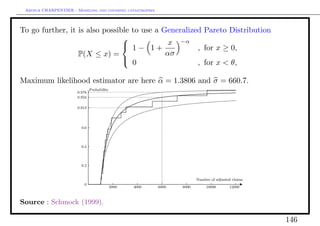
A natural idea is to fit a generalized Pareto distribution for claims exceeding u,
for some u large enough.
threshold [1] 3, we chose u = 3
p.less.thresh [1] 0.9271357, i.e. we keep to 8.5% largest claims
n.exceed [1] 87
method [1] ‘‘ml’’, we use the maximum likelihood technique,
par.ests, we get estimators ξ and σ,
xi sigma
0.6179447 2.0453168
par.ses, with the following standard errors
xi sigma
0.1769205 0.4008392
29](https://image.slidesharecdn.com/slides-saopaulo-catastrophe1-130312204751-phpapp02/85/Slides-saopaulo-catastrophe-1-29-320.jpg)


![Arthur CHARPENTIER - Modeling and covering catastrophes
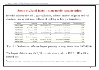
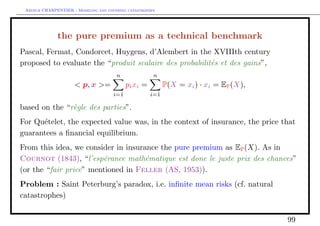
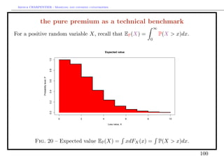
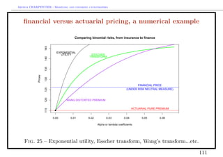
from pure premium to expected utility principle
Ru (X) = u(x)dP = P(u(X) > x))dx
where u : [0, ∞) → [0, ∞) is a utility function.
Example with an exponential utility, u(x) = [1 − e−αx ]/α,
1
Ru (X) = log EP (eαX ) ,
α
i.e. the entropic risk measure.
See Cramer (1728), Bernoulli (1738), von Neumann & Morgenstern
(PUP, 1944), ... etc.
101](https://image.slidesharecdn.com/slides-saopaulo-catastrophe1-130312204751-phpapp02/85/Slides-saopaulo-catastrophe-1-101-320.jpg)
![Arthur CHARPENTIER - Modeling and covering catastrophes
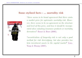
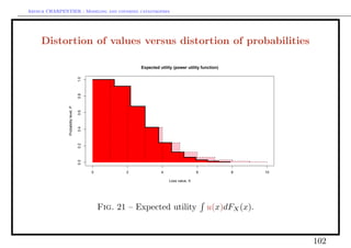
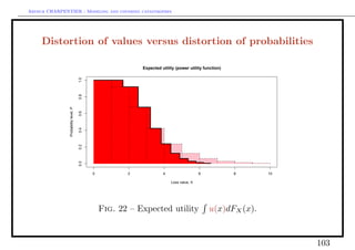
from pure premium to distorted premiums (Wang)
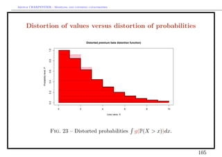
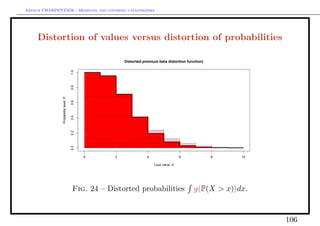
Rg (X) = xdg ◦ P = g(P(X > x))dx
where g : [0, 1] → [0, 1] is a distorted function.
Example
• if g(x) = I(X ≥ 1 − α) Rg (X) = V aR(X, α),
• if g(x) = min{x/(1 − α), 1} Rg (X) = T V aR(X, α) (also called expected
shortfall), Rg (X) = EP (X|X > V aR(X, α)).
See D’Alembert (1754), Schmeidler (PAMS, 1986, E, 1989), Yaari (E, 1987),
Denneberg (KAP, 1994)... etc.
Remark : Rg (X) will be denoted Eg◦P . But it is not an expected value since
Q = g ◦ P is not a probability measure.
104](https://image.slidesharecdn.com/slides-saopaulo-catastrophe1-130312204751-phpapp02/85/Slides-saopaulo-catastrophe-1-104-320.jpg)
![Arthur CHARPENTIER - Modeling and covering catastrophes
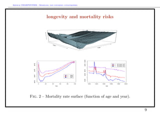
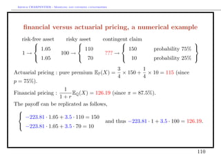
pricing options in complete markets : the binomial case
The only solution of the system is
Cu − Cd 1 Cu − Cd
β= and α = Cu − S0 u .
S0 u − S0 d 1+r S0 u − S0 d
C0 is the price at time 0 of that portfolio.
1 1+r−d
C0 = α + βS0 = (πCu + (1 − π) Cd ) where π = (∈ [0, 1]).
1+r u−d
C1
Hence C0 = EQ where Q is the probability measure (π, 1 − π), called risk
1+r
neutral probability measure.
109](https://image.slidesharecdn.com/slides-saopaulo-catastrophe1-130312204751-phpapp02/85/Slides-saopaulo-catastrophe-1-109-320.jpg)
![Arthur CHARPENTIER - Modeling and covering catastrophes
Cat bonds versus (traditional) reinsurance : the price
• Using distorted premiums (Wang (2000,2002))
If F (x) = P(X > x) denotes the losses survival distribution, the pure premium is
∞
π(X) = E(X) = 0 F (x)dx. The distorted premium is
∞
πg (X) = g(F (x))dx,
0
where g : [0, 1] → [0, 1] is increasing, with g(0) = 0 and g(1) = 1.
Example The proportional hazards (PH) transform is obtained when g is a
power function.
Wang (2000) proposed the following transformation, g(·) = Φ(Φ−1 (F (·)) + λ),
where Φ is the N (0, 1) cdf, and λ is the “market price of risk”, i.e. the Sharpe
ratio. More generally, consider g(·) = tκ (t−1 (F (·)) + λ), where tκ is the Student t
κ
cdf with κ degrees of freedom.
120](https://image.slidesharecdn.com/slides-saopaulo-catastrophe1-130312204751-phpapp02/85/Slides-saopaulo-catastrophe-1-120-320.jpg)

![Arthur CHARPENTIER - Modeling and covering catastrophes
Thus
X
α2 = .
X −θ
Asymptotical properties are then
α(α − 1)2
E(α2 ) → α et V ar(α2 ) → .
n(α − 2)
• OLS regression,
If the logarithm of survival probabilities log[1 − F (x)] are linear in log x, i.e.
log[1 − F (x)] = log F (x) = β0 + β1 log x,
we obtain a Pareto distribution. In that case
Yi = log[1 − F (Xi )] = log F (Xi ) = β0 + β1 log Xi + εi .
The OLS estimator for β = (β0 , β1 ) is then
n n n
−n i=1 log Xi · log F (Xi ) + i=1 log Xi · i=1 log F (Xi )
β1 = −α3 = n n 2
n 2 −
i=1 [log Xi ] [ i=1 log Xi ]
142](https://image.slidesharecdn.com/slides-saopaulo-catastrophe1-130312204751-phpapp02/85/Slides-saopaulo-catastrophe-1-142-320.jpg)
![Arthur CHARPENTIER - Modeling and covering catastrophes
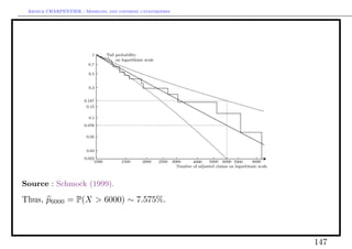
In that case, p6000 = P(X > 6000) ∼ 6−1.37 ∼ 8.57%. It is also possible to derive
bounds for this probability,
p6000 ∈ [4.5%; 16.2%] with 68% chance.
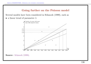
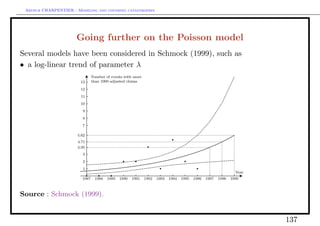
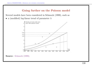
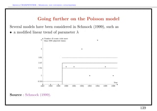
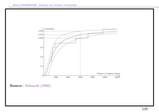
Source : Schmock (1999).
145](https://image.slidesharecdn.com/slides-saopaulo-catastrophe1-130312204751-phpapp02/85/Slides-saopaulo-catastrophe-1-145-320.jpg)
![Arthur CHARPENTIER - Modeling and covering catastrophes
Insurance market intensity λ1
Consider an homogeneous Poisson process with intensity λ1 . Under the
non-artbitrage framework, the compounded discount actuarial fair insurance
price at time t = 0, in the reinsurance market is
3 3
H = E 450 · 1 (τ < 3) e−rτ τ = 450 e−rt t fτ (t)dt = 450 e−rt t λ1 e−λ1 t dt
0 0
i.e. the insurance premium is equal to the value of the expected discounted loss
from earthquake.
With constant interest rate, rt = log(1.0541). Thus
3
26 = 450 e− log(1.0541)t λ1 e−λ1 t dt, where 1 − e−λ1 t is the probability of
0
occurence of an event over period [0, t]. Hence, we get an intensity rate from the
reinsurance market λ1 ≈ 0.0214.
The probability of having (at least) one event in three years is 0.0624, i.e. 2.15
events in one hundred years.
157](https://image.slidesharecdn.com/slides-saopaulo-catastrophe1-130312204751-phpapp02/85/Slides-saopaulo-catastrophe-1-157-320.jpg)
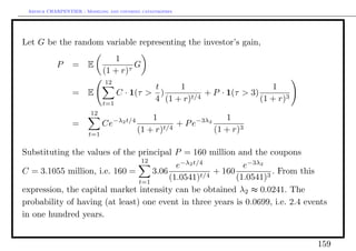

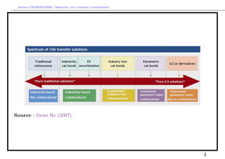
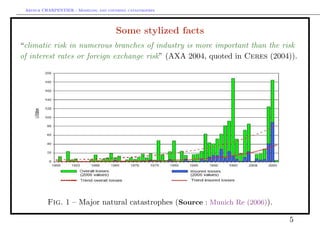
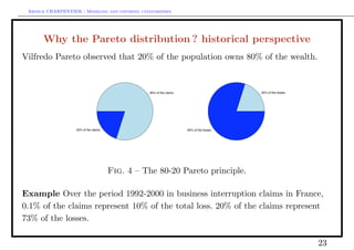
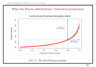
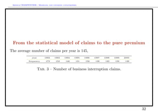
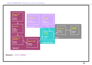
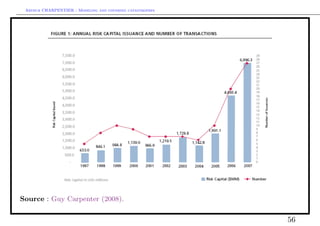
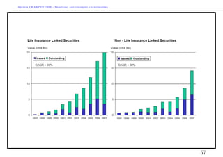
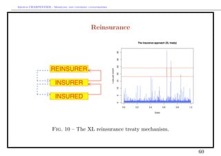
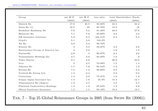
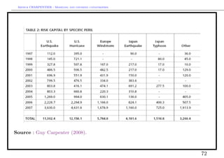
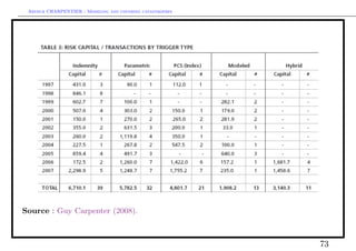
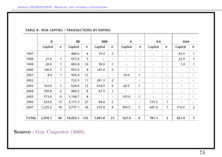
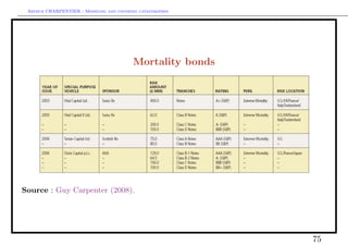
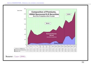
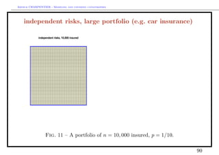
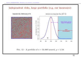
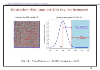
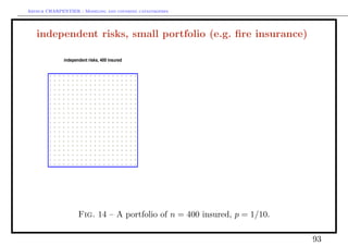
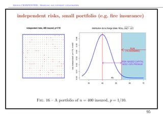
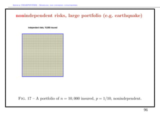
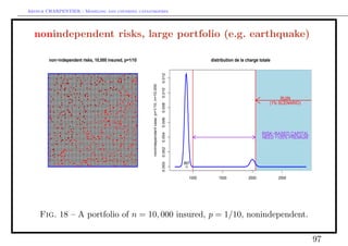
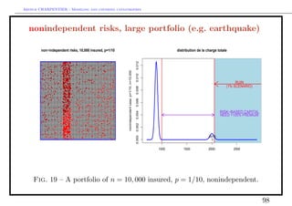
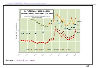
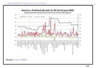
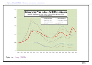
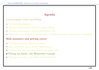
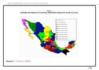
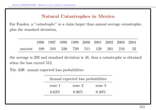
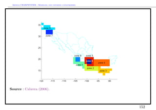
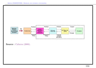
This document discusses modeling and covering catastrophic risks. It begins with an agenda covering catastrophic risk products and models, including modeling very large claims and natural catastrophe accumulation risk. It also discusses insurance covers for catastrophes using both traditional and alternative techniques. The document then discusses risk measures and pricing covers, including pricing insurance-linked securities and calculating risk measures for catastrophic risks. Examples are provided of pricing cat bonds. Throughout, the document provides statistics on catastrophic events such as hurricanes, earthquakes, and industrial accidents, and discusses related concepts such as defining large claims and catastrophic impacts.


