

![Arthur CHARPENTIER - Gestion des risques bancaires et financiers.
Introduction the risk measures, and risk perception
S. Clam [...] once said: I dene a coward as someone who will not bet when
you oer him two-to-one odds and let him choose his side .
With the centuries old St. Petersburg paradox in my mind, I pedantically
corrected him: You mean will not make a suciently small bet (so that the
change in the marginal utility of money will not contaminate his choice). .
Recalling this conversation, a few years ago I oered some lunch colleagues to
bet each $200 to $100 that the side of a coin they specied would not appear at
the rst tom. One distinguished scholar - who lays no claim to advanced
mathematical skills - gave the following answer:
48](https://image.slidesharecdn.com/slides-edf-1-130617053457-phpapp01/85/Slides-edf-1-48-320.jpg)
![Arthur CHARPENTIER - Gestion des risques bancaires et financiers.
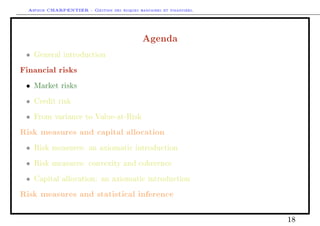
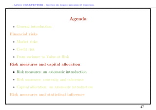
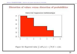
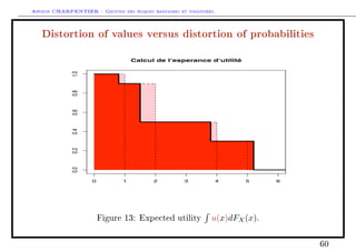
Risk measures: the expected utility approach
Ru(X) = u(x)dP = P(u(X) x))dx
where u : [0, ∞) → [0, ∞) is a utility function.
Example with an exponential utility, u(x) = [1 − e−αx
]/α,
Ru(X) =
1
α
log EP(eαX
) .
55](https://image.slidesharecdn.com/slides-edf-1-130617053457-phpapp01/85/Slides-edf-1-55-320.jpg)
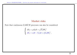
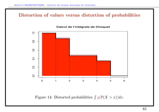
![Arthur CHARPENTIER - Gestion des risques bancaires et financiers.
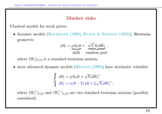
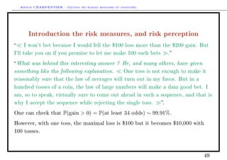
Risk measures: Yarri's dual approach
Rg(X) = xdg ◦ P = g(P(X x))dx
where g : [0, 1] → [0, 1] is a distorted function.
Example if g(x) = I(X ≥ α) Rg(X) = V aR(X, α), and if g(x) = min{x/α, 1}
Rg(X) = TV aR(X, α) (also called expected shortfall),
Rg(X) = EP(X|X V aR(X, α)).
56](https://image.slidesharecdn.com/slides-edf-1-130617053457-phpapp01/85/Slides-edf-1-56-320.jpg)
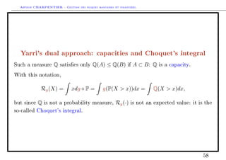
![Arthur CHARPENTIER - Gestion des risques bancaires et financiers.
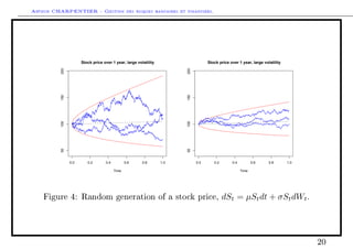
Yarri's dual approach: capacities and Choquet's integral
Here Rg(X) = g(P(X x))dx = g(FX(x))dx with g : [0, 1] → [0, 1]
increasing. Thus, g ◦ FX is a decreasing function taking values in [0, 1] on [0, ∞):
g ◦ FX is a survival function.
Can Rg(X) be seen as an expected value of X with a change of measure ?
Yes if there exists a probability measure Q such that g ◦ FX(x) = Q(X x). If it
is possible to dene such a measure Q, generally Q is not a probability measure.
In fact, Q satises
• Q(∅) = 0 (since FX(∞) = 0 and g(0) = 0),
• Q(Ω) = 1 (since FX(0) = 1 and g(1) = 1),
• Q(A) ≤ Q(B) if A ⊂ B (since FX(·) is decreasing and g(·) is increasing).
57](https://image.slidesharecdn.com/slides-edf-1-130617053457-phpapp01/85/Slides-edf-1-57-320.jpg)
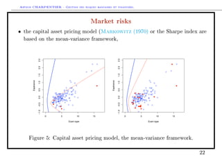
![Arthur CHARPENTIER - Gestion des risques bancaires et financiers.
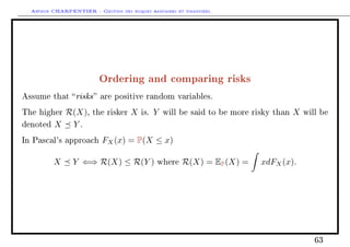
Axiomatic approach for risk measures
There are three way to describe risk measure: characterizing natural properties
that should satisfy
• the risk measure R(·), e.g. R(·) is subadditive (R(X + Y ) ≤ R(X) + R(Y )),
• induced stochastic ordering , i.e. X Y (Y is more risky than X) if and
only if R(X) ≤ R(Y ) [Economics],
• induced set of acceptable risks A, i.e. X ∈ A (X is is acceptable) if and
only if R(X) ≤ 0 [Financial Mathematics].
62](https://image.slidesharecdn.com/slides-edf-1-130617053457-phpapp01/85/Slides-edf-1-62-320.jpg)
![Arthur CHARPENTIER - Gestion des risques bancaires et financiers.
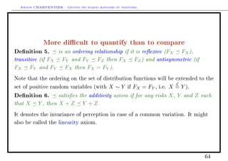
More dicult to quantify than to compare
Denition 7. satises the continuity axiom (or Archimedean axiom) if for
any FX, FY and FZ such that FX FY FZ, then for all α, β ∈ (0, 1)
αFX + [1 − α]FZ FY βFX + [1 − β]FZ.
Proposition 8. If satises the continuity and associativity axioms,
X Y ⇐⇒ R(X) ≤ R(Y )
where
R(X) = EP(X) = xdFX(x) =
∞
0
P(X x)dx.
65](https://image.slidesharecdn.com/slides-edf-1-130617053457-phpapp01/85/Slides-edf-1-65-320.jpg)
![Arthur CHARPENTIER - Gestion des risques bancaires et financiers.
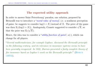
The expected utility approach
Denition 9. satises the independence axiom if for any distribution function
FX, FY and FZ such that FX FY , then for all λ ∈ [0, 1]
λFX + [1 − λ]FZ λFX + [1 − λ]FZ.
or equivalently
(λX) ⊕ ([1 − λ]Z) (λY ) ⊕ ([1 − λ]Z),
where ⊕ denotes a mixture.
Hence, ordering are not modied when mixing risks with a third one. Recall that
(λX) ⊕ ([1 − λ]Z) = (λX) + ([1 − λ]Z).
67](https://image.slidesharecdn.com/slides-edf-1-130617053457-phpapp01/85/Slides-edf-1-67-320.jpg)
![Arthur CHARPENTIER - Gestion des risques bancaires et financiers.
The expected utility approach
The insurance premium is then obtained by the null utility principle: π(X)
satises
EP(u(π(X) − X)) = 0.
Example 12. With an exponential utility, u(x) = [1 − e−αx
]/α, alors
π(X) =
1
α
log EP(eαX
) .
Note that the exponential utility does not exist for heavy tailed risks.
Example 13. With a quadratic utility, u(x) = x − x2
/2s where x s, then
π(X) ∼ EP(X) +
κ
2
V arP(X).
70](https://image.slidesharecdn.com/slides-edf-1-130617053457-phpapp01/85/Slides-edf-1-70-320.jpg)
![Arthur CHARPENTIER - Gestion des risques bancaires et financiers.
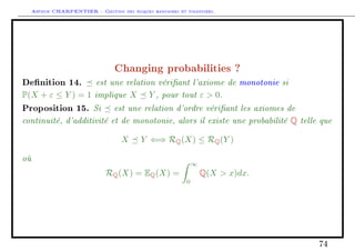
Changing probabilities ?
Le prix de l'option aujourd'hui s'écrit
α + βS0 =
1
1 + r
1 + r − d
u − d
Cu +
u − (1 + r)
u − d
Cd ,
qui peut s'écrire
π =
1
1 + r
(qCu + (1 − q)Cd) , où q =
1 + r − d
u − d
.
Notons que q ∈ [0, 1], c'est à dire que le prix de l'option est l'espérance
mathématique, sous une probabilité Q appelée probabilité risque neutre du payo
à échéance: π = EQ (payo). Notons que Q n'a rien n'a voir avec la probabilité
dite historique P qu'a le sous-jacent de monter ou de descendre: le prix d'un
payo aléatoire X ne s'écrit pas EP (X).
78](https://image.slidesharecdn.com/slides-edf-1-130617053457-phpapp01/85/Slides-edf-1-78-320.jpg)
![Arthur CHARPENTIER - Gestion des risques bancaires et financiers.
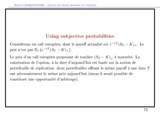
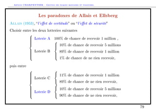
La distortion de probabilités, Yaari (1987)
Example 16. Un exemple de relation d'ordre est la dominance stochastique à
l'ordre 1. X 1 Y si et seulement si une des conditions suivantes (équivalentes)
sont satisfaites,
• E(g(X)) ≤ E(g(Y )) pour g croissante,
• pour tout x ∈ R, P(X ≤ x) ≥ P(Y ≤ x),
• pour tout x ∈ R, P(X x) ≤ P(Y x),
• pour tout x ∈]0, 1[, V aR(X, α) ≤ V aR(Y, α).
Cette relation d'ordre est notée V aR dans Denuit Charpentier (2004).
Example 17. Un exemple de relation d'ordre est la dominance stochastique à
l'ordre 2. X 2 Y si et seulement si une des conditions suivantes (équivalentes)
sont satisfaites,
• E(g(X)) ≤ E(g(Y )) pour g croissante et convexe,
• E((X − t)+) ≤ E((Y − t)+) pour t ∈ R,
81](https://image.slidesharecdn.com/slides-edf-1-130617053457-phpapp01/85/Slides-edf-1-81-320.jpg)
![Arthur CHARPENTIER - Gestion des risques bancaires et financiers.
• pour tout x ∈]0, 1[,
α
0
V aR(X, p)dp ≥
α
0
V aR(Y, p)dp,
• pour tout x ∈]0, 1[,
∞
α
V aR(X, p)dp ≤
∞
α
V aR(Y, p)dp,
• pour tout x ∈ [0, 1[, TV aR(X, α) ≤ TV aR(Y, α).
Cette relation d'ordre est notée T V aR dans Denuit Charpentier (2004).
Denition 18. est une relation vériant l'axiome d'indépendance comonotone
si X Y implique X + Z Y + Z pour tout Z tel que les couples (X, Z) et
(Y, Z) soient comonotones.
Remark 19. X et Z sont comonotones s'il n'existe pas ω, ω tels que
X(ω) X(ω ) et Y (ω) Y (ω ).
Denition 20. est une relation vériant l'axiome de cohérence si pour des
variables X et Y constantes (P(X = x) = P(Y = y) = 1), FX FY implique
x ≤ y.
82](https://image.slidesharecdn.com/slides-edf-1-130617053457-phpapp01/85/Slides-edf-1-82-320.jpg)
![Arthur CHARPENTIER - Gestion des risques bancaires et financiers.
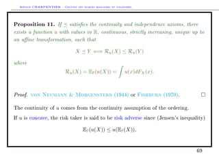
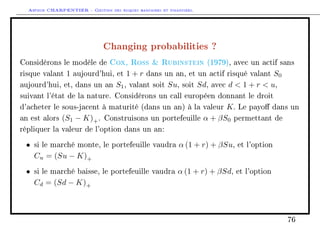
Proposition 21. Si est une relation d'ordre vériant les axiomes de
continuité, d'indépendance comonotone, monotonie, et est compatible avec la
dominance stochastique à l'ordre 1, alors il existe une unique fonction de
distortion croissante g : [0, 1] → [0, 1] telle que
X Y ⇐⇒ Rg(X) ≤ Rg(Y )
où
Rg(X) = xdg ◦ P = g(P(X x))dx =
1
0
F−1
X (1 − p)dg(p).
83](https://image.slidesharecdn.com/slides-edf-1-130617053457-phpapp01/85/Slides-edf-1-83-320.jpg)
![Arthur CHARPENTIER - Gestion des risques bancaires et financiers.
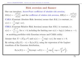
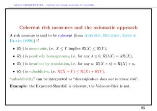
Convex risk measures
A risk measure is said to be convex (from Artzner, Delbaen, Eber Heath
(1999)) if
• R(·) is monotonic, i.e. X ≤ Y implies R(X) ≤ R(Y ),
• R(·) is invariant by translation, i.e. for any κ, R(X + κ) = R(X) + κ,
• R(·) is convex, i.e. R(λX + (1 − λ)Y ) ≤ λR(X) + (1 − λ)R(Y ), for any
λ ∈ [0, 1].
Hence, if a convex measure satises the homogeneity condition, it is coherent.
Remark A natural way to dene a convex measure satisfying the small size
coherent condition is adding a coherent measure a liquidity charge,
Rconvex(X) = Rcoherent(X) + Cliquidity(X).
86](https://image.slidesharecdn.com/slides-edf-1-130617053457-phpapp01/85/Slides-edf-1-86-320.jpg)
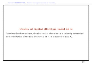
![Arthur CHARPENTIER - Gestion des risques bancaires et financiers.
Capital allocation based on Shapley value
One idea is to use the Shapley value.
Let Si denote all the subsets of {1, 2, ..., n} that contain i.
The Shapley-value of risk i is
ki =
S∈Si
(|s| − 1)!)(n − |s|)!
n!
· [Γ(S) − Γ(S {i})],
where | · | denote the size of the subset (cardinality).
It is simply a weighted average of all possible congurations.
Note that here k1 + ... + kn = k.
This capital allocation has been used by Swiss Re.
94](https://image.slidesharecdn.com/slides-edf-1-130617053457-phpapp01/85/Slides-edf-1-94-320.jpg)
![Arthur CHARPENTIER - Gestion des risques bancaires et financiers.
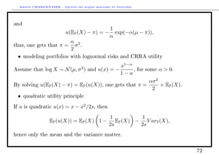
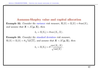
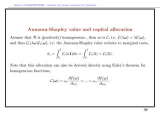
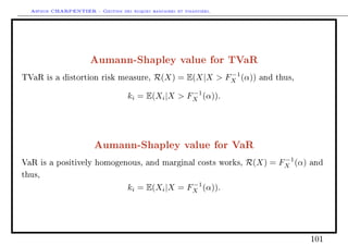
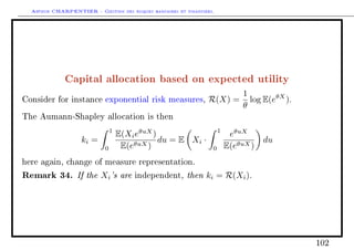
Capital allocation based on Aumann-Shapley value
An alternative is to use the Aumann-Shapley value.
Here the idea is to consider sensitivity of marginal cost. Dene the following cost
function, C : [0, 1]n
→ R,
C(ω) = R(ωt
X) = R
n
i=1
ωiXi .
Note that C(1) = R(X) = k.
Dene Ci(ω) =
∂C(ω)
∂ωi
, and dene the Aumann-Shapley value as
ki =
1
0
Ci(u1)du.
96](https://image.slidesharecdn.com/slides-edf-1-130617053457-phpapp01/85/Slides-edf-1-96-320.jpg)
![Arthur CHARPENTIER - Gestion des risques bancaires et financiers.
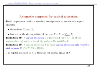
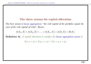
Capital allocation and decision loss function
Capital allocation can also be seen as the solution of distance minimization
problem.
Consider some distance d(ki, Xi|R, k, X). Then
ki = argminκ(κ, Xi|R, k, X).
Example 35. Consider the following expected value distance,
d(ki, Xi) = E([Xi − ki]2
).
Then ki =
k
n
+ E(Xi) −
E(X)
n
.
Example 36. Consider the following tail VaR distance,
d(ki, Xi|α, k, X) = E([Xi − ki]2
|X F−1
X (α)).
Then ki =
k
n
+ E(Xi|X F−1
X (α)) −
E(X|X F−1
X (α))
n
.
103](https://image.slidesharecdn.com/slides-edf-1-130617053457-phpapp01/85/Slides-edf-1-103-320.jpg)
![Arthur CHARPENTIER - Gestion des risques bancaires et financiers.
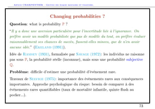
Example 37. Consider the following stop loss distance,
d(ki, Xi) = E([Xi − ki]+).
Then ki = F−1
Xi
(FX+ (k)).
Example 38. Consider the following distance on risk measures,
d(ki, Xi) = R(Xi) −
ki
k
(R(X1) + ... + R(Xn))
2
.
Then ki =
R(Xi)
R(X1) + ... + R(Xn)
· k.
104](https://image.slidesharecdn.com/slides-edf-1-130617053457-phpapp01/85/Slides-edf-1-104-320.jpg)
![Arthur CHARPENTIER - Gestion des risques bancaires et financiers.
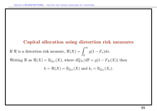
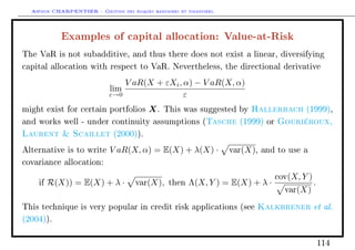
And nally a similar idea is to write V aR(X, α) = TV aR(X, a(X)) for some a(·)
with values in [0, 1], and to consider capital allocation based on TVaR (see
Overbeck (2000)).
Numerical example based on a simulated portfolio
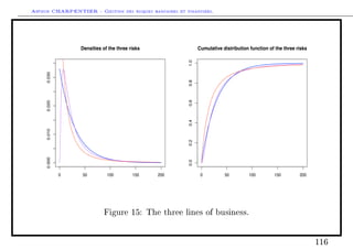
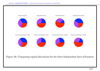
Consider three lines of business, with rather dierent behaviors,
• an exponential distribution X1 ∼ E(0.03), E(X1) ∼ 33,
• a log-normal distribution X2 ∼ LN(3, 1), E(X2) ∼ 33,
• a Pareto distribution X3 ∼ P(2, 30), E(X3) ∼ 33,
Assume further that the three risks are independent.
115](https://image.slidesharecdn.com/slides-edf-1-130617053457-phpapp01/85/Slides-edf-1-115-320.jpg)
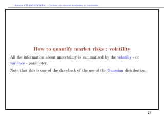
![Arthur CHARPENTIER - Gestion des risques bancaires et financiers.
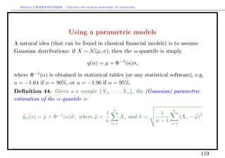
Using a parametric models
Actually, is the Gaussian model does not t very well, it is still possible to use
Gaussian approximation
If the variance is nite, (X − E(X))/σ might be closer to the Gaussian
distribution, and thus, consider the so-called Cornish-Fisher approximation (see
[?] or [?]), i.e.
Q(X, α) ∼ E(X) + zα V (X), (1)
where
zα = Φ−1
(α)+
ζ1
6
[Φ−1
(α)2
−1]+
ζ2
24
[Φ−1
(α)3
−3Φ−1
(α)]−
ζ2
1
36
[2Φ−1
(α)3
−5Φ−1
(α)],
(2)
where ζ1istheskewnessofX, andζ2
is the excess kurtosis, i.e. i.e.
ζ1 =
E([X − E(X)]3
)
E([X − E(X)]2)3/2
and ζ1 =
E([X − E(X)]4
)
E([X − E(X)]2)2
− 3. (3)
120](https://image.slidesharecdn.com/slides-edf-1-130617053457-phpapp01/85/Slides-edf-1-120-320.jpg)
![Arthur CHARPENTIER - Gestion des risques bancaires et financiers.
Using a parametric models
Denition 45. Given a n sample {X1, · · · , Xn}, the Cornish-Fisher estimation
of the α-quantile is
qn(α) = µ + zασ, where µ =
1
n
n
i=1
Xi and σ =
1
n − 1
n
i=1
(Xi − µ)
2
,
and
zα = Φ−1
(α)+
ζ1
6
[Φ−1
(α)2
−1]+
ζ2
24
[Φ−1
(α)3
−3Φ−1
(α)]−
ζ2
1
36
[2Φ−1
(α)3
−5Φ−1
(α)],
where ζ1 is the natural estimator for the skewness of X, and ζ2
is the natural
estimator of the excess kurtosis, i.e. ζ1 =
n(n − 1)
n − 2
√
n
n
i=1(Xi − µ)3
(
n
i=1(Xi − µ)2)
3/2
and
ζ2 = n−1
(n−2)(n−3) (n + 1)ζ2 + 6 whereζ2 =
n n
i=1(Xi−µ)4
( n
i=1(Xi−µ)2
)
2 − 3.
121](https://image.slidesharecdn.com/slides-edf-1-130617053457-phpapp01/85/Slides-edf-1-121-320.jpg)
![Arthur CHARPENTIER - Gestion des risques bancaires et financiers.
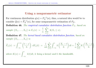
Smoothing nonparametric estimators
Two techniques have been considered to smooth estimation of quantiles, either
implicit, or explicit.
• consider a linear combinaison of order statistics,
The classical empirical quantile estimate is simply
Qn (p) = F−1
n
i
n
= X(i) = X([np]) where [·] denotes the integer part. (5)
The estimator is simple to obtain, but depends only on one observation. A
natural extention will be to use - at least - two observations, if np is not an
integer. The weighted empirical quantile estimate is then dened as
Qn (p) = (1 − γ) X([np]) + γX([np]+1) where γ = np − [np] .
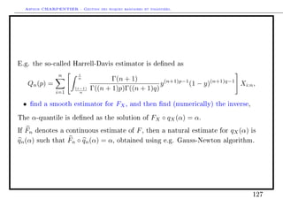
124](https://image.slidesharecdn.com/slides-edf-1-130617053457-phpapp01/85/Slides-edf-1-124-320.jpg)

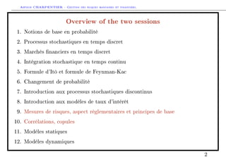
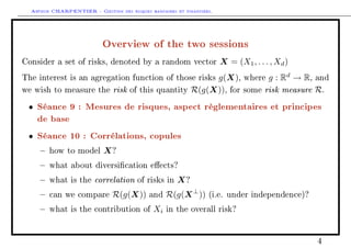
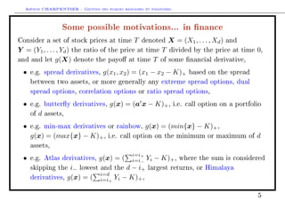
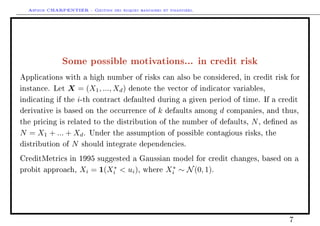
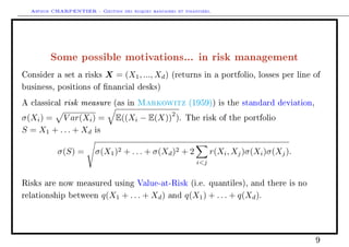
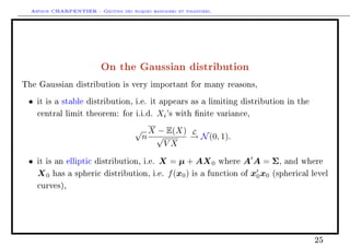
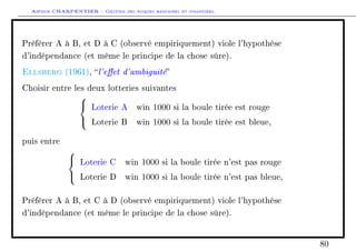
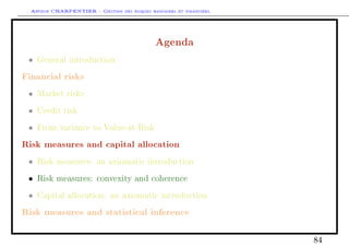
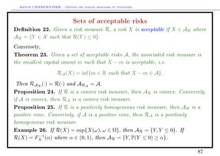
The document outlines two sessions on risk management in banking and finance. Session 9 will cover risk measures, regulatory aspects, and basic principles, including defining risk measures, academic vs accounting standards, desirable properties, and estimating risks from samples. Session 10 will cover correlations, copulas, modeling dependencies between risks, diversification effects, comparing risks under dependence vs independence, and analyzing individual risk contributions. Examples of applications to finance, environmental risks, and credit risk are also provided.


![[Lehman brothers] interest rate parity, money market basis swaps, and cross c...](https://cdn.slidesharecdn.com/ss_thumbnails/lehmanbrothersinterestrateparitymoneymarketbasisswapsandcross-currencybasisswaps-120814082308-phpapp01-thumbnail.jpg?width=640&height=640&fit=bounds)


