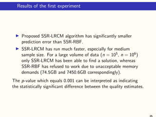
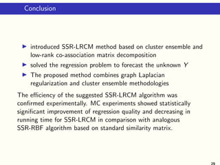
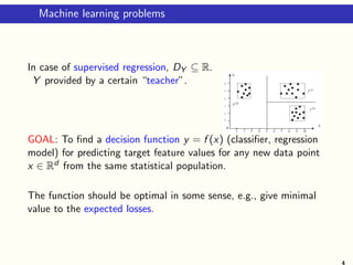
This document summarizes a semi-supervised regression method that combines graph Laplacian regularization with cluster ensemble methodology. It proposes using a weighted averaged co-association matrix from the cluster ensemble as the similarity matrix in graph Laplacian regularization. The method (SSR-LRCM) finds a low-rank approximation of the co-association matrix to efficiently solve the regression problem. Experimental results on synthetic and real-world datasets show SSR-LRCM achieves significantly better prediction accuracy than an alternative method, while also having lower computational costs for large datasets. Future work will explore using a hierarchical matrix approximation instead of low-rank.

1. Semi-Supervised Regression using Cluster
Ensemble
Alexander Litvinenko1
,
joint work with
Vladimir Berikov2,3
1
RWTH Aachen, 2
Sobolev Institute of Mathematics, and 3
Novosibirsk
State University, Russia
Crete

2. Plan
After reviewing ML problems, we
introduce semi-supervised ML problem
propose a method which combines graph Laplacian
regularization and cluster ensemble methodologies
solve a semi-supervised regression problem
demonstrate 2 numerical examples.

3. Machine learning (ML) problems
Let X = {x1, . . . , xn} be a given data set.
And xi ∈ Rd be a feature vector.
ML problems can be classified as
supervised,
unsupervised,
semi-supervised.
In a supervised learning context, we are given an additional set
Y = {y1, . . . , yn} of target feature values (labels) for all data
points, yi ∈ DY , where DY is target feature domain.
DY is an unordered set of categorical values (classes, patterns).
3

4. Machine learning problems
In case of supervised regression, DY ⊆ R.
Y provided by a certain “teacher”.
GOAL: To find a decision function y = f (x) (classifier, regression
model) for predicting target feature values for any new data point
x ∈ Rd from the same statistical population.
The function should be optimal in some sense, e.g., give minimal
value to the expected losses.
4

5. Unsupervised learning setting
The target feature values are not provided.
Example: the problem of cluster analysis, consists in finding a
partition P = {C1, . . . , CK } of X.
The desired number of clusters is either a predefined parameter or
should be found in the best way.
5

6. Semi-supervised learning problems
The target feature values are known only for a part of data set
X1 ⊂ X.
Example: manual annotation of digital images is rather time-consuming.
Assume that X1 = {x1, . . . , xn1 }, and the unlabeled part is X0 = {xn1+1, . . . , xn}.
The set of labels for points from X1 is denoted by Y1 = {y1, . . . , yn1 }.
GOAL: Predict target feature values as accurately as possible either for given
unlabeled data X0 (i.e., perform transductive learning) or for arbitrary new
observations from the same statistical population (inductive learning).
To improve prediction accuracy, we use information contained in both labeled
and unlabeled data.

7. Further Plan of this work
solve a semi-supervised regression problem.
propose a novel semi-supervised regression method using a
combination of graph Laplacian regularization technique and
cluster ensemble methodology.
Ensemble clustering aims at finding consensus partition of
data using some base clustering algorithms.

8. Combined semi-supervised regression and ensemble clustering
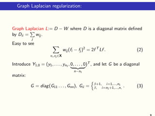
Graph Laplacian regularization:
find f ∗ such that f ∗ = arg min
f ∈Rn
Q(f ), where
Q(f ) :=
1
2


xi ∈X1
(fi − yi )2
+ α
xi ,xj ∈X
wij (fi − fj )2
+ β||f ||2

 ,
(1)
f = (f1, . . . , fn) is a vector of predicted outputs: fi = f (xi );
α, β > 0 are regularization parameters,
W = (wij ) is data similarity matrix, e.g. Mat´ern family:
W (h) = σ2
2ν−1Γ(ν)
h ν
Kν
h
with three parameters , ν, and σ2.
[1st term in (1) minimizes fitting error on labeled data; the 2nd term aims to
obtain ”smooth” predictions on both labeled and unlabeled sample; 3rd - is
Tikhonov’s regularizer]
8

9. Graph Laplacian regularization:
Graph Laplacian L:= D − W where D is a diagonal matrix defined
by Dii =
j
wij .
Easy to see
xi ,xj ∈X
wij (fi − fj )2
= 2f T
Lf . (2)
Introduce Y1,0 = (y1, . . . , yn1 , 0, . . . , 0
n−n1
)T , and let G be a diagonal
matrix:
G = diag(G11 . . . , Gnn), Gii = β+1, i=1,...,n1
β, i=n1+1,...,n, . (3)
9

10. Graph Laplacian regularization:
Differentiating Q(f ) with respect to f , we get
∂Q
∂f
|f =f ∗ = Gf ∗
+ αLf ∗
− Y1,0 = 0,
hence
f ∗
= (G + αL)−1
Y1,0 (4)
under the condition that the inverse of matrix sum exists (note
that the regularization parameters α, β can be selected to guaranty
the well-posedness of the problem).
10

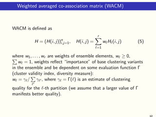
11. Co-association matrix of cluster ensemble
Use a co-association matrix of cluster ensemble as similarity matrix
in (1).
Let us consider a set of partition variants {P }r
=1, where
P = {C ,1, . . . , C ,K }, C ,k ⊂ X,
C ,k C ,k = ∅,
K is number of clusters in -th partition.
For each P we determine matrix H = (h (i, j))n
i,j=1 with elements
indicating whether a pair xi , xj belong to the same cluster in -th
variant or not:
h (i, j) = I[c (xi ) = c (xj )], where
I(·) is indicator function (I[true] = 1, I[false] = 0),
c (x) is cluster label assigned to x.
11

12. Weighted averaged co-association matrix (WACM)
WACM is defined as
H = (H(i, j))n
i,j=1, H(i, j) =
r
=1
w H (i, j) (5)
where w1, . . . , wr are weights of ensemble elements, w ≥ 0,
w = 1, weights reflect “importance” of base clustering variants
in the ensemble and be dependent on some evaluation function Γ
(cluster validity index, diversity measure):
w = γ / γ , where γ = Γ( ) is an estimate of clustering
quality for the -th partition (we assume that a larger value of Γ
manifests better quality).
12

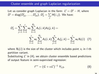
13. Low-rank approximation of WACM
Proposition 1. Weighted averaged co-association matrix admits
low-rank decomposition in the form:
H = BBT
, B = [B1B2 . . . Br ] (6)
where B is a block matrix, B =
√
w A , A is (n × K ) cluster
assignment matrix for -th partition: A (i, k) = I[c(xi ) = k],
i = 1, . . . , n, k = 1, . . . , K .
13

14. Cluster ensemble and graph Laplacian regularization
Let us consider graph Laplacian in the form: L = D − H, where
D = diag(D11, . . . , Dnn), Dii =
j
H(i, j). We have:
Dii =
n
j=1
r
=1
w
K
k=1
A (i, k)A (j, k) =
r
=1
w
K
k=1
A (i, k)
n
j=1
Al (j, k) =
r
=1
w N (i) (7)
where N (i) is the size of the cluster which includes point xi in -th
partition variant.
Substituting L in (4), we obtain cluster ensemble based predictions
of output feature in semi-supervised regression:
f ∗∗
= (G + αL )−1
Y1,0. (8)
14

15. Using law-rank representation of H, we get:
f ∗∗
= (G + αD − αBBT
)−1
Y1,0.
In linear algebra, the following Woodbury matrix identity is known:
(S + UV )−1
= S−1
− S−1
U(I + VS−1
U)−1
VS−1
where S ∈ Rn×n is invertible matrix, U ∈ Rn×m and V ∈ Rm×n.
We can denote S = G + αD and get
S−1
= diag(1/(G11 + αD11), . . . , 1/(Gnn + αDnn)) (9)
where Gii , Dii , i = 1, . . . , n are defined in (3) and (7)
correspondingly.

16. Proposition 2. Cluster ensemble based target feature prediction
vector (8) can be calculated using low-rank decomposition as
follows:
f ∗∗
= (S−1
+ αS−1
B(I − αBT
S−1
B)−1
BS−1
) Y1,0 (10)
where matrix B is defined in (6) and S−1 in (9).
In (10) we invert (m × m) matrix instead of (n × n) in (8).
Total cost of (10) is O(nm + m3).
16

17. Algorithm SSR-LRCM
Input:
X: dataset including both labeled and unlabeled sample;
Y1: target feature values for labeled instances;
r: number of runs for base clustering algorithm µ;
Ω: set of parameters (working conditions) of clustering algorithm.
Output:
f ∗∗: predictions of target feature for labeled and unlabeled objects.
17

18. Construction of the consensus partition
18

19. Algorithm SSR-LRCM
Steps:
1. Generate r variants of clustering partition with algorithm µ for
working parameters randomly chosen from Ω; calculate
weights w1, . . . , wr of variants.
2. Find graph Laplacian in law-rank representation using
matrices B in (6) and D in (7);
3. Calculate predictions of target feature according to (10).
end.
In the implementation of SSR-LRCM, we use K-means as base
clustering algorithm
19

20. Numerics
Aim: to confirm the usefulness of involving cluster ensemble for
similarity matrix estimation in semi-supervised regression.
Evaluate the regression quality on a synthetic and a real-life
example.
20

21. First example with two clusters and artificial noisy data
Datasets generated from a mixture of N(a1, σX I) and N(a2, σX I)
under equal weights;
a1, a2 ∈ Rd , d = 8, σX is a parameter.
Let
Y = 1 + ε for points generated from N(a1, σX I),
Y = 2 + ε otherwise, ε ∈ N(0, σ2
ε ).
To study robustness of the algorithm, we also generate two
independent random variables following uniform distribution
U(0, σX ) and use them as additional “noisy” features.
21

22. First example with two clusters and artificial noisy data
In MC modeling, we repeatedly generate samples of size n
according to the given distribution mixture.
labeled sample = 10% randomly selected
unlabeled sample = 90%.
Also vary parameter σε for the target feature.
In SSR-LRCM, use K-means as a base clustering algorithm. The
ensemble variants are designed by random initialization of
centroids (#clusters=2).
r = 10, weights w ≡ 1/r.
regul. params α, β estimated using grid search and cross-validation
technique.
(best results for α = 1, β = 0.001, and σX = 5).

23. First example with two clusters and artificial noisy data
For the comparison purposes, we consider the method (denoted as
SSS-RBF) which uses the standard similarity matrix evaluated with
RBF kernel.
The quality of prediction is estimated as
Root Mean Squared Error:
RMSE = 1
n (ytrue
i − fi )2,
where ytrue
i is a true value.
To make the results more statistically sound, we have averaged
error estimates over 40 MC repetitions and compare the results by
paired two sample Student’s t-test.
23

24. Results of experiments with a mixture of two distributions.
Significantly different RMSE values (p-value < 10−5) are in bold.
For n = 105 and n = 106, SSR-RBF failed due to unacceptable
memory demands.
n σε
SSR-LRCM SSR-RBF
RMSE tens (sec) tmatr (sec) RMSE time (sec)
1000
0.01 0.052 0.06 0.02 0.085 0.10
0.1 0.054 0.04 0.04 0.085 0.07
0.25 0.060 0.04 0.04 0.102 0.07
3000
0.01 0.049 0.06 0.02 0.145 0.74
0.1 0.051 0.06 0.02 0.143 0.75
0.25 0.053 0.07 0.02 0.150 0.79
7000
0.01 0.050 0.16 0.08 0.228 5.70
0.1 0.050 0.16 0.08 0.229 5.63
0.25 0.051 0.14 0.07 0.227 5.66
105
0.01 0.051 1.51 0.50 - -
106
0.01 0.051 17.7 6.68 - -
24

25. Results of the first experiment
Proposed SSR-LRCM algorithm has significantly smaller
prediction error than SSR-RBF.
SSR-LRCM has run much faster, especially for medium
sample size. For a large volume of data (n = 105, n = 106)
only SSR-LRCM has been able to find a solution, whereas
SSR-RBF has refused to work due to unacceptable memory
demands (74.5GB and 7450.6GB correspondingly).
The p-value which equals 0.001 can be interpreted as indicating
the statistically significant difference between the quality estimates.

26. Second example with 10-dimensional real Forest Fires dataset
GOAL: predict burned area of forest fires, in the northeast region
of Portugal, by using meteorological and other information.
Fire Weather Index (FWI) System is applied to get feature values.
FWI is based on daily observations of temperature, relative
humidity, wind speed, and 24-hour rainfall. Numerical features:
X,Y-axis spatial coordinate within the Montesinho park map;
Fine Fuel Moisture Code;
Duff Moisture Code;
Initial Spread Index;
Drought Code;
temperature in Celsius degrees;
relative humidity;
wind speed in km/h;
outside rain in mm/m2;
the burned area of the forest in ha (predicted feature).
26

27. Second example
This problem above is known as a difficult regression task, in which
the best RMSE was attained by the naive mean predictor.
We use quantile regression approach:
the transformed quartile value of response feature should be
predicted.
27

28. Second example
Volume of labeled sample is 10% of overall data;
K-means base algorithm with 10 clusters with ensemble size
r = 10 is used.
α = 1, β = 0.001, SSR-RBF parameter = 0.1.
The number of generations of the labeled samples is 40.
Results: averaged error rate
for SSR-LRCM is RMSE= 1.65,
for SSR-RBF is RMSE = 1.68.
28

29. Conclusion
introduced SSR-LRCM method based on cluster ensemble and
low-rank co-association matrix decomposition
solved the regression problem to forecast the unknown Y
The proposed method combines graph Laplacian
regularization and cluster ensemble methodologies
The efficiency of the suggested SSR-LRCM algorithm was
confirmed experimentally. MC experiments showed statistically
significant improvement of regression quality and decreasing in
running time for SSR-LRCM in comparison with analogous
SSR-RBF algorithm based on standard similarity matrix.

30. Future work
Instead of a low-rank approximation of the weighted averaged
co-association matrix H = BBT (or W ), we will use a hierarchical
(H-) matrix approximation of H (W ) and then solve for f ∗∗:
f ∗∗
= (G + αD − α ˜H)−1
Y1,0.
in the H-matrix format.
54
54
86
86
68
67 67
20
39 112
48 73
15 39
112
112 123
63 107
56 65
107
107
82
67 67
25
50
67
58 66
59 58
71 76
50 75
16 41
66
66 73
63 63
62 66
63
63 67
84
58 67
54 55
75 76
69
60 60
59 60
56 55
79
63 63
65
70
58 63
59 57
67 69
63 80
64
64 79
59 66
54 56
66
66 66
82
57 65
60 66
79 83
65
65 70
112 112
19
43
76
82 112
73 72
62 83
37 51
12 32
79
71 71
115 115
87 115
78 77
127
127
66
66 67
63
73 125
70 77
59 75
125
125
81
64 64
76 125
78 84
125
125
65
65 73
48
71
79
56 65
61 67
75 82
59 71
43 61
65
65 82
59 70
54 60
70
60 60
80
52 60
48 54
67 52
71
64 64
54 61
61 55
61
61 70
69
74
48 59
52 63
67 67
64 78
59
59 85
119 119
64 119
65 74
70
62 62
120 120
12
29
45
47
59 120
51 58
53 69
44 52
25 40
8 20
80
67 67
46 65
50 56
65
64 64
67 122
62 61
122
122 122
69
71 113
63 71
58 71
113
113
74
74 84
64 104
59 72
104
104 120
55
69
63 120
66 80
66 74
43 60
78
57 57
125 125
81 125
69 78
62
62 77
122 122
68
77 122
62 65
64 81
122
122 123
76 123
71 80
70
63 63
63 63
56 55
75
65 65
34
56
73
85
70 65
63 60
76 93
55 61
45 54
27 40
78
66 66
124 124
68 123
63 71
123
123
66
66 70
61
69 127
68 74
60 74
127
127
77
63 63
73 123
63 74
123
123
61
61 82
57
72
66 123
67 88
63 74
45 61
123
113 113
72 113
65 75
73
59 59
62 59
59 57
76
76 79
69
68
52 62
54 64
72 83
62 74
62
62 73
58 69
62 58
69
66 66
83 123
26 26
123
26 26
An example of the H-matrix approximation of W
30

31. Literature
1. V. Berikov, I. Pestunov, Ensemble clustering based on weighted
co-association matrices: Error bound and convergence properties, Pattern
Recognition. 2017. Vol. 63. P. 427-436.
2. V. Berikov, A. Litvinenko, Semi-Supervised Regression using Cluster
Ensemble and Low-Rank Co-Association Matrix Decomposition under
Uncertainties, arXiv:1901.03919, (2019).
3. V. Berikov, N. Karaev, A. Tewari, Semi-supervised classification with
cluster ensemble. In Engineering, Computer and Information Sciences
(SIBIRCON), International Multi-Conference. 245-250. IEEE. (2017)
4. V.B. Berikov, Construction of an optimal collective decision in cluster
analysis on the basis of an averaged co-association matrix and cluster
validity indices. Pattern Recognition and Image Analysis. 27(2), 153-165
(2017)
5. V.B. Berikov, A. Litvinenko, The influence of prior knowledge on the
expected performance of a classifier. Pattern recognition letters 24 (15),
2537-2548, (2003)
6. V Berikov, A Litvinenko, Methods for statistical data analysis with
decision trees, Novosibirsk,
http://www.math.nsc.ru/AP/datamine/eng/context.pdf, Sobolev
Institute of Mathematics, 2003

32. Acknowledgements
The research was partly supported by
1. Scientific research program “Mathematical methods of pattern recognition
and prediction” in the Sobolev Institute of Mathematics SB RAS.
2. Russian Foundation for Basic Research grants 18-07-00600,
18-29-0904mk, 19-29-01175
3. Russian Ministry of Science and Education under the 5-100 Excellence
Programme.
4. A. Litvinenko by funding from the Alexander von Humboldt Foundation.
32