Downloaded 120 times

![Multi-image vs. Single-image
Multi-image
Source: [Park et al. SPM 2003]
Single-image
Source: [Freeman et al. CG&A 2002]](https://image.slidesharecdn.com/singleimagesuper-resolutionfromtransformedself-exemplarscvpr2015-150613221257-lva1-app6891/85/Single-Image-Super-Resolution-from-Transformed-Self-Exemplars-CVPR-2015-3-320.jpg)
![External Example-based Super-Resolution
Learning to map from low-res to high-res patches
• Nearest neighbor [Freeman et al. CG&A 02]
• Neighborhood embedding [Chang et a. CVPR 04]
• Sparse representation [Yang et al. TIP 10]
• Kernel ridge regression [Kim and Kwon PAMI 10]
• Locally-linear regression [Yang and Yang ICCV 13] [Timofte et al. ACCV 14]
• Convolutional neural network [Dong et al. ECCV 14]
• Random forest [Schulter et al. CVPR 15]
External dictionary](https://image.slidesharecdn.com/singleimagesuper-resolutionfromtransformedself-exemplarscvpr2015-150613221257-lva1-app6891/85/Single-Image-Super-Resolution-from-Transformed-Self-Exemplars-CVPR-2015-4-320.jpg)
![Internal Example-based Super-Resolution
Low-res and high-res example pairs from patch
recurrence across scale
• Non-local means with self-examples [Ebrahimi and Vrscay ICIRA 2007]
• Unified classical and example SR [Glasner et al. ICCV 2009]
• Local self-similarity [Freedman and Fattal TOG 2011]
• In-place regression [Yang et al. ICCV 2013]
• Nonparametric blind SR [Michaeli and Irani ICCV 2013]
• SR for noisy images [Singh et al. CVPR 2014]
• Sub-band self-similarity [Singh et al. ACCV 2014]
Internal dictionary](https://image.slidesharecdn.com/singleimagesuper-resolutionfromtransformedself-exemplarscvpr2015-150613221257-lva1-app6891/85/Single-Image-Super-Resolution-from-Transformed-Self-Exemplars-CVPR-2015-5-320.jpg)
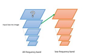
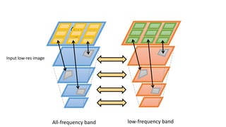
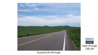
![Input low-res image
All-frequency band low-frequency band
Super-Resolution Scheme
Multi-scale version of [Freedman and Fattal TOG 2011]](https://image.slidesharecdn.com/singleimagesuper-resolutionfromtransformedself-exemplarscvpr2015-150613221257-lva1-app6891/85/Single-Image-Super-Resolution-from-Transformed-Self-Exemplars-CVPR-2015-10-320.jpg)
![Input low-res image
LR/HR example pairs
Super-Resolution Scheme
Multi-scale version of [Freedman and Fattal TOG 2011]
low-frequency bandAll-frequency band](https://image.slidesharecdn.com/singleimagesuper-resolutionfromtransformedself-exemplarscvpr2015-150613221257-lva1-app6891/85/Single-Image-Super-Resolution-from-Transformed-Self-Exemplars-CVPR-2015-11-320.jpg)
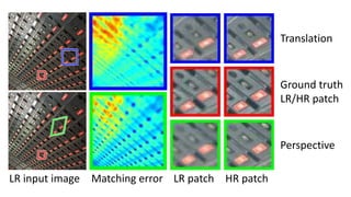
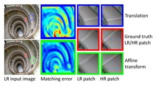
![Super-Resolution as Nearest Neighbor Field Estimation
Appearance cost Plane compatibility Scale cost
[Huang et al. SIGGRAPH 2014] Scale](https://image.slidesharecdn.com/singleimagesuper-resolutionfromtransformedself-exemplarscvpr2015-150613221257-lva1-app6891/85/Single-Image-Super-Resolution-from-Transformed-Self-Exemplars-CVPR-2015-14-320.jpg)
![Search Patch Transformation
• Generalized PatchMatch [Barnes et al. ECCV 2010]
• Randomization
• Spatial propagation
• Backward compatible when planar structures were not detected
Perspective Similarity Affine
[Huang et al. SIGGRAPH 2014]](https://image.slidesharecdn.com/singleimagesuper-resolutionfromtransformedself-exemplarscvpr2015-150613221257-lva1-app6891/85/Single-Image-Super-Resolution-from-Transformed-Self-Exemplars-CVPR-2015-15-320.jpg)

![Dataset – Set5, Set14, and Sun-Hays 80
Set5
Set 14 Sun-Hays 80 [Sun and Hays ICCP 12]](https://image.slidesharecdn.com/singleimagesuper-resolutionfromtransformedself-exemplarscvpr2015-150613221257-lva1-app6891/85/Single-Image-Super-Resolution-from-Transformed-Self-Exemplars-CVPR-2015-18-320.jpg)
![Ground-truth HR
SRCNN [Dong et al. ECCV 14] Glasner [Glasner et al. ICCV 2009]
Our result
SR Factor 4x
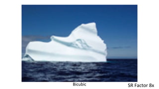
Bicubic
A+ [Timofte et al. ACCV 14]](https://image.slidesharecdn.com/singleimagesuper-resolutionfromtransformedself-exemplarscvpr2015-150613221257-lva1-app6891/85/Single-Image-Super-Resolution-from-Transformed-Self-Exemplars-CVPR-2015-19-320.jpg)
![SR Factor 4x
Ground-truth HR
SRCNN [Dong et al. ECCV 14] Glasner [Glasner et al. ICCV 2009]
Our result
Bicubic
A+ [Timofte et al. ACCV 14]](https://image.slidesharecdn.com/singleimagesuper-resolutionfromtransformedself-exemplarscvpr2015-150613221257-lva1-app6891/85/Single-Image-Super-Resolution-from-Transformed-Self-Exemplars-CVPR-2015-20-320.jpg)
![SR Factor 4x
Ground-truth HR
SRCNN [Dong et al. ECCV 14] Glasner [Glasner et al. ICCV 2009]
Our result
Bicubic
A+ [Timofte et al. ACCV 14]](https://image.slidesharecdn.com/singleimagesuper-resolutionfromtransformedself-exemplarscvpr2015-150613221257-lva1-app6891/85/Single-Image-Super-Resolution-from-Transformed-Self-Exemplars-CVPR-2015-21-320.jpg)
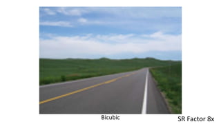
![Bicubic
SRCNN [Dong et al. ECCV 14] A+ [Timofte et al. ACCV 14]
Our result
Ground-truth HR
Sub-band [Singh et al. ACCV 2014]](https://image.slidesharecdn.com/singleimagesuper-resolutionfromtransformedself-exemplarscvpr2015-150613221257-lva1-app6891/85/Single-Image-Super-Resolution-from-Transformed-Self-Exemplars-CVPR-2015-22-320.jpg)
![Ground-truth
SRCNN [Dong et al. ECCV 14]
Glasner [Glasner et al. ICCV 2009]
Our result](https://image.slidesharecdn.com/singleimagesuper-resolutionfromtransformedself-exemplarscvpr2015-150613221257-lva1-app6891/85/Single-Image-Super-Resolution-from-Transformed-Self-Exemplars-CVPR-2015-23-320.jpg)
![Ground-truth HR
SRCNN [Dong et al. ECCV 14]
Glasner [Glasner et al. ICCV 2009]
Our result](https://image.slidesharecdn.com/singleimagesuper-resolutionfromtransformedself-exemplarscvpr2015-150613221257-lva1-app6891/85/Single-Image-Super-Resolution-from-Transformed-Self-Exemplars-CVPR-2015-24-320.jpg)
![Bicubic
SRCNN [Dong et al. ECCV 14] A+ [Timofte et al. ACCV 14]
Our result
Ground-truth HR
Sub-band [Singh et al. ACCV 2014]](https://image.slidesharecdn.com/singleimagesuper-resolutionfromtransformedself-exemplarscvpr2015-150613221257-lva1-app6891/85/Single-Image-Super-Resolution-from-Transformed-Self-Exemplars-CVPR-2015-25-320.jpg)
![Bicubic
SRCNN [Dong et al. ECCV 14] A+ [Timofte et al. ACCV 14]
Our result
Ground-truth HR
Our resultSub-band [Singh et al. ACCV 2014]](https://image.slidesharecdn.com/singleimagesuper-resolutionfromtransformedself-exemplarscvpr2015-150613221257-lva1-app6891/85/Single-Image-Super-Resolution-from-Transformed-Self-Exemplars-CVPR-2015-26-320.jpg)
![Bicubic
SRCNN [Dong et al. ECCV 14] A+ [Timofte et al. ACCV 14]
Our result
Ground-truth HR
Glasner [Glasner et al. ICCV 2009]](https://image.slidesharecdn.com/singleimagesuper-resolutionfromtransformedself-exemplarscvpr2015-150613221257-lva1-app6891/85/Single-Image-Super-Resolution-from-Transformed-Self-Exemplars-CVPR-2015-27-320.jpg)
![Bicubic
SRCNN [Dong et al. ECCV 14] A+ [Timofte et al. ACCV 14]
Our result
Ground-truth HR
ScSR [Yang et al. TIP 10]](https://image.slidesharecdn.com/singleimagesuper-resolutionfromtransformedself-exemplarscvpr2015-150613221257-lva1-app6891/85/Single-Image-Super-Resolution-from-Transformed-Self-Exemplars-CVPR-2015-28-320.jpg)
![Bicubic
SRCNN [Dong et al. ECCV 14] A+ [Timofte et al. ACCV 14]
Our result
Ground-truth HR
ScSR [Yang et al. TIP 10]](https://image.slidesharecdn.com/singleimagesuper-resolutionfromtransformedself-exemplarscvpr2015-150613221257-lva1-app6891/85/Single-Image-Super-Resolution-from-Transformed-Self-Exemplars-CVPR-2015-29-320.jpg)
![Bicubic
SRCNN [Dong et al. ECCV 14] A+ [Timofte et al. ACCV 14]
Our result
Ground-truth HR
ScSR [Yang et al. TIP 10]](https://image.slidesharecdn.com/singleimagesuper-resolutionfromtransformedself-exemplarscvpr2015-150613221257-lva1-app6891/85/Single-Image-Super-Resolution-from-Transformed-Self-Exemplars-CVPR-2015-30-320.jpg)
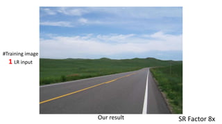
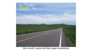
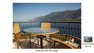
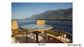
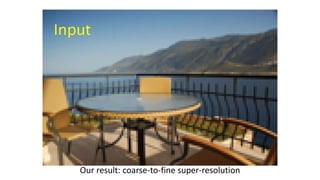
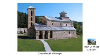
![Internet-scale scene matching [Sun and Hays ICCP 12] SR Factor 8x
#Training images
6.3 millions](https://image.slidesharecdn.com/singleimagesuper-resolutionfromtransformedself-exemplarscvpr2015-150613221257-lva1-app6891/85/Single-Image-Super-Resolution-from-Transformed-Self-Exemplars-CVPR-2015-36-320.jpg)
![SRCNN [Dong et al. ECCV 14] SR Factor 8x
#Training images
395,909
from ImageNet](https://image.slidesharecdn.com/singleimagesuper-resolutionfromtransformedself-exemplarscvpr2015-150613221257-lva1-app6891/85/Single-Image-Super-Resolution-from-Transformed-Self-Exemplars-CVPR-2015-37-320.jpg)
![Sparse coding [Yang et al. TIP 10] SR Factor 8x](https://image.slidesharecdn.com/singleimagesuper-resolutionfromtransformedself-exemplarscvpr2015-150613221257-lva1-app6891/85/Single-Image-Super-Resolution-from-Transformed-Self-Exemplars-CVPR-2015-42-320.jpg)
![SRCNN [Dong et al. ECCV 14] SR Factor 8x](https://image.slidesharecdn.com/singleimagesuper-resolutionfromtransformedself-exemplarscvpr2015-150613221257-lva1-app6891/85/Single-Image-Super-Resolution-from-Transformed-Self-Exemplars-CVPR-2015-43-320.jpg)


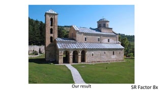
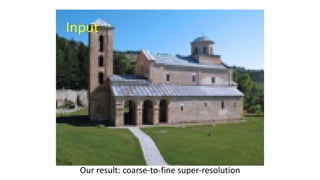
![SR Factor 8xInternet-scale scene matching [Sun and Hays ICCP 12]](https://image.slidesharecdn.com/singleimagesuper-resolutionfromtransformedself-exemplarscvpr2015-150613221257-lva1-app6891/85/Single-Image-Super-Resolution-from-Transformed-Self-Exemplars-CVPR-2015-48-320.jpg)
![SR Factor 8xSRCNN [Dong et al. ECCV 14]](https://image.slidesharecdn.com/singleimagesuper-resolutionfromtransformedself-exemplarscvpr2015-150613221257-lva1-app6891/85/Single-Image-Super-Resolution-from-Transformed-Self-Exemplars-CVPR-2015-49-320.jpg)
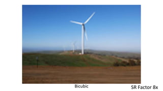
![SRCNN [Dong ECCV 2014] SR Factor 8x](https://image.slidesharecdn.com/singleimagesuper-resolutionfromtransformedself-exemplarscvpr2015-150613221257-lva1-app6891/85/Single-Image-Super-Resolution-from-Transformed-Self-Exemplars-CVPR-2015-53-320.jpg)

![SRCNN [Dong ECCV 2014] SR Factor 8x](https://image.slidesharecdn.com/singleimagesuper-resolutionfromtransformedself-exemplarscvpr2015-150613221257-lva1-app6891/85/Single-Image-Super-Resolution-from-Transformed-Self-Exemplars-CVPR-2015-56-320.jpg)

![Low-Res
TI-DTV
[Fernandez-Granda
and Candes ICCV 2013]
Ours
SR Factor 4x](https://image.slidesharecdn.com/singleimagesuper-resolutionfromtransformedself-exemplarscvpr2015-150613221257-lva1-app6891/85/Single-Image-Super-Resolution-from-Transformed-Self-Exemplars-CVPR-2015-58-320.jpg)
![Low-Res
TI-DTV
[Fernandez-Granda
and Candes ICCV 2013]
Ours
SR Factor 4x](https://image.slidesharecdn.com/singleimagesuper-resolutionfromtransformedself-exemplarscvpr2015-150613221257-lva1-app6891/85/Single-Image-Super-Resolution-from-Transformed-Self-Exemplars-CVPR-2015-59-320.jpg)
![Limitations – Blur Kernel Model
• Suffer from blur kernel mismatch
• Blind SR to estimate kernel
[Michaeli and Irani ICCV 2013]
[Efrat et al. ICCV 2013]
• With ground truth kernel, we can
get significantly improvement
• External example-based method
would need to retrain the model](https://image.slidesharecdn.com/singleimagesuper-resolutionfromtransformedself-exemplarscvpr2015-150613221257-lva1-app6891/85/Single-Image-Super-Resolution-from-Transformed-Self-Exemplars-CVPR-2015-60-320.jpg)
![Limitations
• Slow computation time
• On average, 40 seconds for super-resolving 2x on an image in BSD 100 dataset
on a 2.8Ghz PC, 12G RAM PC
SRF 4x
Ground truth HR Our result
A+ [Timofte et al. ACCV 14]SRCNN [Dong et al. ECCV 14]](https://image.slidesharecdn.com/singleimagesuper-resolutionfromtransformedself-exemplarscvpr2015-150613221257-lva1-app6891/85/Single-Image-Super-Resolution-from-Transformed-Self-Exemplars-CVPR-2015-61-320.jpg)
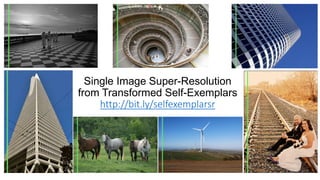

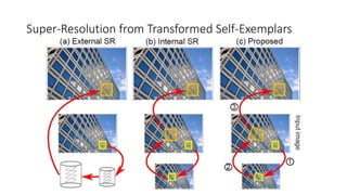
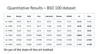
The document discusses a method for single image super-resolution using transformed self-exemplars, aiming to recover high-resolution images from low-resolution inputs without requiring external training data. It outlines various techniques and results, demonstrating improvements in performance on multiple datasets compared to state-of-the-art methods. The approach shows particular effectiveness for urban scenes, achieving comparable results while avoiding complex learning algorithms.


![[OSGeo-KR Tech Workshop] Deep Learning for Single Image Super-Resolution](https://cdn.slidesharecdn.com/ss_thumbnails/osgeo-krdeeplearningforsingleimagesuper-resolution-180223175347-thumbnail.jpg?width=640&height=640&fit=bounds)


![“zero-shot” super-resolution using deep internal learning [CVPR2018]](https://cdn.slidesharecdn.com/ss_thumbnails/cvpr2018zero-shotsuper-resolutionusingdeepinternallearning-210903045317-thumbnail.jpg?width=640&height=640&fit=bounds)