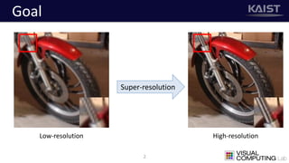
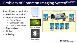
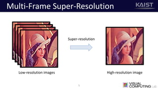
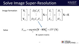
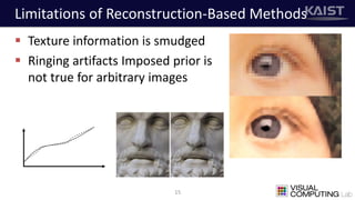
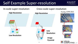
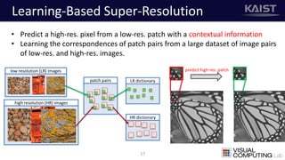
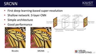
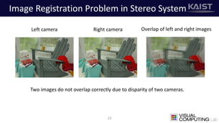
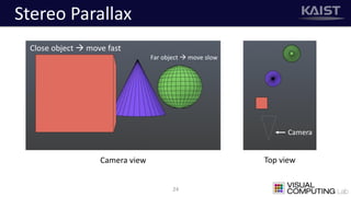
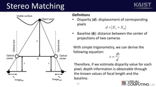
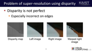
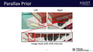
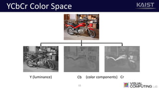
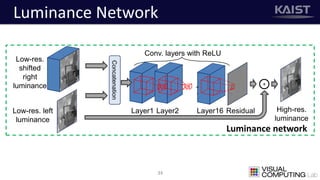
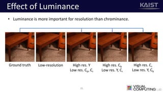
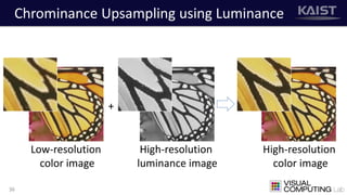
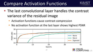
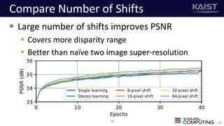
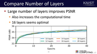
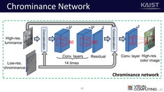
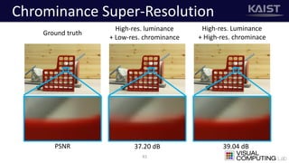
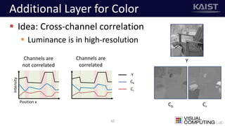
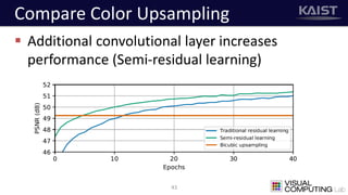
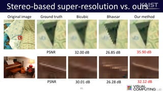
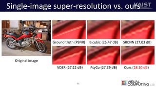
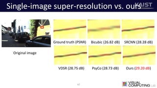
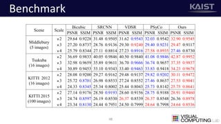
The document discusses a deep learning-based approach for stereo super-resolution, which aims to enhance the spatial resolution of stereo images using a parallax prior. The method addresses common imaging system issues and surpasses traditional techniques by reconstructing high-resolution images without direct disparity calculation, demonstrating promising performance metrics. Results indicate the proposed method outperforms existing state-of-the-art approaches in stereo imaging applications.

1. Deep Learning-Based
Stereo Super-Resolution
전석준, 백승환, 최인창, 김민혁
2018.08.09
Enhancing the Spatial Resolution of Stereo Images using a Parallax Prior
Daniel S. Jeon, Seung-Hwan Baek, Inchang Choi, Min H. Kim
Proc. IEEE Computer Vision and Pattern Recognition (CVPR 2018)
Salt Lake City, USA, June 18, 2018

2. Goal
2
Super-resolution
Low-resolution High-resolution

3. Problem of Common Imaging System
3
loss of spatial resolution
 Pixel discretization
 Optical distortions
 Out of focus
 Diffraction limit
 Optical aberration
 Motion blur
 Noise
 Aliasing
Out of focus
Diffraction
Sensor

4. BACKGROUND
4

5. Multi-Frame Super-Resolution
5
Low-resolution images High-resolution image
Super-resolution

6. Multi-Frame Super-Resolution
6
Sensor 1 Sensor 2 Sensor 3
 Approach
 Sub-pixel Image Registration
 Projection to high-res. grid
Low-res. Images High-res. grid

7. Sub-Pixel Image Registration
7
Image 1 Image 2 Cross-correlation

8. Sub-Pixel Image Registration
8
 Estimate sub-pixel shift in high-res. grid
In low-res. grid
In high-res. grid

9. Degradation Model
9
High-resolution
image
X
Warp 1
F1
Warp N
FN
Warp 2
F2
Blur 1
C1
Blur 2
C2
Blur N
CN
Decimate 1
D1
Decimate 2
D2
Decimate N
DN
……….
……….
……….
∑
∑
∑
Noise 1
Noise 2
Noise N
1Y
2Y
3Y
Low-resolution
images
Decimation: systematic degradation of spatial resolution

10. Solve Image Super-Resolution
10
1 1 1 1 1 1
N N N N N N
D C F E H
D C F E H
       
                 
              
Y
X X E
Y
Image formation
 
2
2
arg minMAP
X
X TV  Y HX XSolve
H: system matrix

11. Limitation of Traditional SR
 Needs precise (subpixel accuracy) motion estimates.
 Long capture time due to multiple frame acquisition.
 Subject should not move.
11

12. RELATED WORK
12

13. Single-Image Super-Resolution
Single-Image
Super-Resolution
Interpolation-
Based
Reconstruction-
Based
Exemplar-
Based
Internal
Learning
External
Learning
13
• Bilinear
• Bicubic
• Lanczos

14. Reconstruction-Based Methods
 Main idea: Preserve edge information
14
Sun et al., CVPR 2008 Fattal, SIGGRAPH 2007

15. Limitations of Reconstruction-Based Methods
 Texture information is smudged
 Ringing artifacts Imposed prior is
not true for arbitrary images
15

16. Self Example Super-resolution
16
Low Resolution
High Resolution
Low
Resolution
High Resolution
Image
Pyramid
In-scale super-resolution Cross-scale super-resolution
Huang, CVPR 2015

17. Learning-Based Super-Resolution
17
• Predict a high-res. pixel from a low-res. patch with a contextual information
• Learning the correspondences of patch pairs from a large dataset of image pairs
of low-res. and high-res. images.
predict high-res. patchlow resolution (LR) images
high resolution (HR) images
patch pairs LR dictionary
HR dictionary

18. SRCNN
 First deep learning-based super-resolution
 Shallow network: 3-layer CNN
 Simple architecture
 Good performance
18
Bicubic SRCNN

19. Deep CNN
 Vanishing gradient problem
 Deeper network decreases performance
 End-to-end relation requires very long-term memory
19
3 layers
4 layers
5 layers

20.  Learning difference of low-resolution and high-resolution
 Prevent vanishing gradient problem
Residual Learning
20
Low-resolution
color image
High-resolution
color image
-
Residual (sparse)
Kaiming He et al., 2015

21. Residual Learning Model
 Skip connection to learn residual only
 64 channels, 3×3 filters in each convolutional layer
 20 convolutional layers (41×41 receptive field)
21
Interpolated LR HR
Skip-connection way
learned residualConv.1 Conv.D-1ReLu.1 ReLu.D-1
Kim et al., CVPR 2016

22. OUR METHOD
22

23. Image Registration Problem in Stereo System
23
Left camera Right camera
Two images do not overlap correctly due to disparity of two cameras.
Overlap of left and right images

24. Stereo Parallax
24
Camera view Top view
Close object  move fast
Far object  move slow
Camera

25. Stereo Matching
25
Object point
b
z
Imageleft
Imageright
f f
Visible surface
Opticalaxis
Opticalaxis
xL xR
Optical
center
Optical
center
Definitions
• Disparity (d): displacement of corresponding
pixels
• Baseline (b): distance between the center of
projections of two cameras
With simple trigonometry, we can derive the
following equation:
Therefore, if we estimate disparity value for each
pixel, depth information is obtainable through
the known values of focal length and the
baseline.
L Rd X X 
fb
z
d


26. Problem of super-resolution using disparity
26
Disparity map Left image Warped right
image
Right image
 Disparity is not perfect
 Especially incorrect on edges

27. Parallax Prior
27
Left Right
Image stack with shift intervals

28. Input With Shifted Images
 1 Left Image
 64 shifted right images (1 ~ 64 pixels shift)
28
…
Left image 64 shifted right images

29. Receptive Field
 Receptive Field
 Part of the input that is visible to a neuron
 It increases as we stack more convolutional layers
29
Example) 3×3 kernel with 3 convolutions
 Total 7×7 receptive field size

30. Max Disparity
 Max disparity
 64 shifted images with one-pixel intervals
 16 layers  33×33 receptive field
 Total 80 pixels max disparity
 More than about 98% of disparities in the
Middlebury stereo dataset are with this range
30

31.  60 Middlebury images
 Input
 33×33 patch pairs
 24 stride
 Data augmentation
Dataset
31
Original patch Rotating Flipping

32. Two Network Design
32
Low-res. left
luminance
Low-res.
shifted
right luminance
Low-res. left
chrominance
Luminance
network
Chrominance
network
High-res.
color image
High-res.
luminance
Concatenation

33. YCbCr Color Space
33
Y (luminance) Cb Cr(color components)

34. Luminance Network
34
Low-res. left
luminance
Low-res.
shifted
right
luminance
High-res.
luminance
··
·
Layer1 Layer2 Layer16 Residual
Conv. layers with ReLU
+
Luminance network
Concatenation

35. Effect of Luminance
35
Ground truth Low-resolution High res. Y
Low res. Cb, Cr
High res. Cb
Low res. Y, Cr
High res. Cr
Low res. Y, Cb
• Luminance is more important for resolution than chrominance.

36. Chrominance Upsampling using Luminance
36
+
Low-resolution
color image
High-resolution
luminance image
High-resolution
color image

37. Compare Activation Functions
37
 The last convolutional layer handles the contrast
variance of the residual image
 Activation functions cause contrast compression
 No activation function at the last layer shows highest PSNR

38. Compare Number of Shifts
38
 Large number of shifts improves PSNR
 Covers more disparity range
 Better than naïve two image super-resolution

39. Compare Number of Layers
39
 Large number of layers improves PSNR
 Also increases the computational time
 16 layers seems optimal

40. Chrominance Network
40
Low-res.
chrominance
High-res.
luminance
High-res.
color image
Conv. layers
14 times
Conv. layer
64 3 6
Residual
…
64
Concatenation
Chrominance network
Concatenation

41. Chrominance Super-Resolution
41
Ground truth
High-res. luminance
+ Low-res. chrominance
High-res. Luminance
+ High-res. chrominace
PSNR 37.20 dB 39.04 dB

42. Additional Layer for Color
 Idea: Cross-channel correlation
 Luminance is in high-resolution
42
Position x
Intensity
Y
Cb
Cr
Channels are
not correlated
Channels are
correlated
Y
Cb Cr

43. Compare Color Upsampling
43
 Additional convolutional layer increases
performance (Semi-residual learning)

44. RESULTS
44

45. Stereo-based super-resolution vs. ours
45
PSNR 32.00 dB 26.85 dB 35.90 dB
Ground truth Bicubic Bhavsar Our methodOriginal image
PSNR 30.01 dB 26.28 dB 32.12 dB

46. Single-image super-resolution vs. ours
46
Ground truth (PSNR) Bicubic (25.47 dB) SRCNN (27.03 dB)
VDSR (27.22 dB) PsyCo (27.39 dB) Ours (28.10 dB)
Original image

47. Single-image super-resolution vs. ours
47
Ground truth (PSNR) Bicubic (26.82 dB) SRCNN (28.28 dB)
VDSR (28.75 dB) PsyCo (28.73 dB) Ours (29.20 dB)
Original image

48. Benchmark
48
Scene Scale
Bicubic SRCNN VDSR PSyCo Ours
PSNR SSIM PSNR SSIM PSNR SSIM PSNR SSIM PSNR SSIM
Middlebury
(5 images)
×2 29.64 0.9228 31.48 0.9505 31.62 0.9543 32.03 0.9542 32.90 0.9545
×3 27.20 0.8737 28.76 0.9136 29.30 0.9240 29.40 0.9231 29.47 0.9117
×4 25.79 0.8344 27.11 0.8814 27.23 0.8916 27.58 0.8935 27.46 0.8730
Tsukuba
(16 images)
×2 36.69 0.9833 40.05 0.9846 40.50 0.9840 41.08 0.9846 42.87 0.9952
×3 32.98 0.9659 35.89 0.9611 36.70 0.9666 36.74 0.9657 37.35 0.9837
×4 30.89 0.9453 33.10 0.9343 33.40 0.9463 33.83 0.9418 34.23 0.9678
KITTI 2012
(16 images)
×2 28.08 0.9200 29.27 0.9162 29.48 0.9137 29.82 0.9202 30.11 0.9472
×3 25.72 0.8701 26.98 0.8533 27.24 0.8552 27.46 0.8637 27.53 0.9041
×4 24.33 0.8345 25.34 0.8002 25.44 0.8043 25.73 0.8142 25.75 0.8641
KITTI 2015
(100 images)
×2 27.14 0.9176 28.50 0.9193 28.60 0.9156 28.75 0.9188 28.91 0.9460
×3 24.74 0.8597 26.19 0.8530 26.37 0.8539 26.37 0.8548 26.36 0.8978
×4 23.34 0.8130 24.44 0.7951 24.50 0.7999 24.64 0.7998 24.64 0.8536

49. Conclusion
 Reconstruct a high-resolution image without
direct disparity calculation
 Proposed stereo super-resolution outperforms
current state-of-the-art methods
 It can be used with any other stereo imaging
methods additionally
49