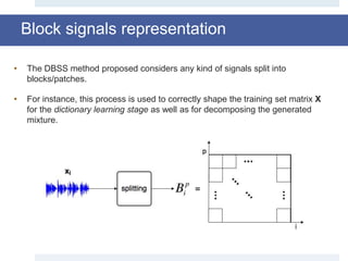
Downloaded 100 times


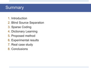
![• Mathematically speaking we say that, since the signal x is a vector and the
dictionary D is a normalized basis, α in Rk is the vector that satisfies the
following optimization problem:
where ψ(α) is the l0 pseudo norm of α.
• In this form the optimization problem is NP-hard [1], but…
aÎÂk
min
1
2
x - Da 2
2
+ ly(a)
Sparse coding (cont.)](https://image.slidesharecdn.com/smpresentation-161025103809/85/Blind-Source-Separation-using-Dictionary-Learning-9-320.jpg)
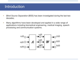
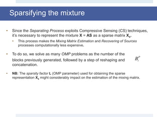
![Orthogonal Matching Pursuit [2]
• Orthogonal Matching Pursuit(OMP) falls into the class of Pursuit Algorithms and
it’s able to identify the “best corresponding projections” of multidimensional data
over the span of a redundant dictionary D.
• Given a matrix of signals X = [x1,…,xn] in Rm×n and a dictionary D = [d1,…,dk] in
Rm×k, the algorithm computes a matrix A = [α1,…,αn] in Rk×n, where for each
column of X, it returns a coefficient vector α which is an approximation solution
of the following NP-hard problem [1]:
aÎÂk
min x - Da 2
2
s.t. a £ L
or
aÎÂk
min a 0
s.t. x - Da 2
2
£e
or
aÎÂk
min
1
2
x - Da 2
2
+ l a 0](https://image.slidesharecdn.com/smpresentation-161025103809/85/Blind-Source-Separation-using-Dictionary-Learning-11-320.jpg)
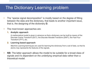
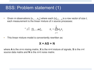
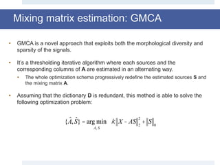
![Dictionary Learning: MOD [3]
• This method views the problem posed in the previous equation as a nested
minimization problem:
1. An inner minimization to find a sparse representation A, given the source signals X
and dictionary D.
2. An outer minimization to find D.
• At the k-th step we have that:
D = D(k-1)
A = OMP(X,D)
• The techniques goes on for a defined number of iterations or until a
convergence criteria is satisfied.
D(k) =
D
argmin X - DA F
2
= XAk
T
(AAk
T
)-1
= XAk
+](https://image.slidesharecdn.com/smpresentation-161025103809/85/Blind-Source-Separation-using-Dictionary-Learning-17-320.jpg)
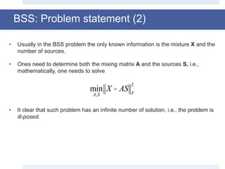
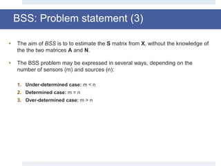
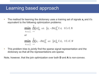
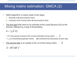
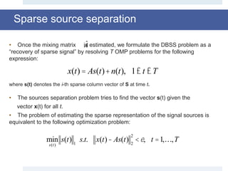
![Mixing matrix estimation
• BSS approach may be divided into two categories:
• Methods which jointly estimate the mixing matrix and the signals and
• methods which first estimate the mixing matrix and then use it to reconstruct the
original signal.
• The method presented here is a two step methods since the separation and
reconstruction processes do not happen within the mixing estimation step.
• Due the lack of an efficient technique for estimating the mixing matrix from a
sparse mixture, here, for this project we’ve used the Generalized
Morphological Component Analysis (GMCA) [4] for estimating the mixing
matrix.](https://image.slidesharecdn.com/smpresentation-161025103809/85/Blind-Source-Separation-using-Dictionary-Learning-19-320.jpg)
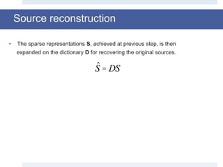
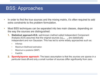
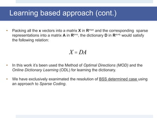
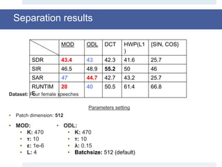
![Experimental results
• Dataset: Sixth Community-Based Signal Separation Evaluation
Campaign, Sisec 2015 [5, 6].
• WAV audio file related to male or female voices and musical
instruments.
• Each source is sampled at16 KHz (160,000 sample), with a duration of 10 sec.
• All the results shown here have been averaged on 10 run, so that the
method could be statistically evaluated.
• The mixing matrix is randomly generated for each test, and the same
matrix is used in each run.](https://image.slidesharecdn.com/smpresentation-161025103809/85/Blind-Source-Separation-using-Dictionary-Learning-24-320.jpg)
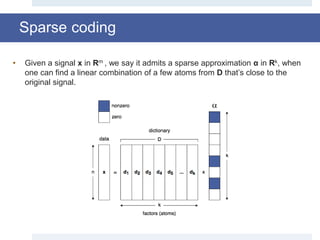
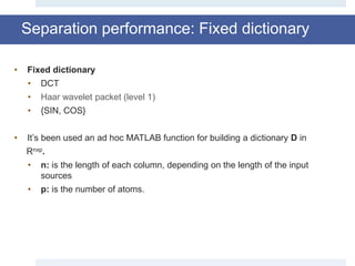
![Evaluation metrics
• For objective quality assessment, we use three performance criteria defined in
the BSSEVAL toolbox [7] to evaluate the estimated source signals.
, e
• The estimated source can be composed as follows:
• According to [7], both SIR and SAR measure local performance,
• while SDR is global performance index, which may give better assessment to
the overall performance of the algorithms under comparison.
SDR =10log
starget
2
einterf +enoise +eartif
2
SIR =10log
starget
2
einterf
2
SAR =10log
starget +einterf +enoise
2
eartif
2](https://image.slidesharecdn.com/smpresentation-161025103809/85/Blind-Source-Separation-using-Dictionary-Learning-25-320.jpg)
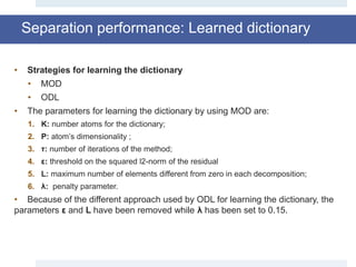
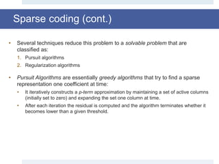
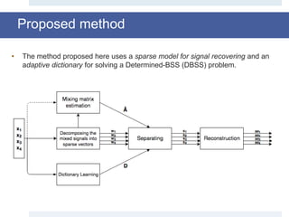
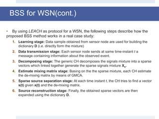
![Real case study: BSS in a Wireless Sensor Network
LEACH [8]
• A Wireless Sensor Network (WSN) is an interconnection of autonomous
sensors that:
1. Collect data from the environment.
2. Relay data through the network to
to a main location.
• Each node may be connect to
several other nodes, thus it may receive
a mixture of signals at its receiver.
• To transmit the message across the
network effectively, it’s necessary for
the receiver to separate the sources
from the mixture.](https://image.slidesharecdn.com/smpresentation-161025103809/85/Blind-Source-Separation-using-Dictionary-Learning-31-320.jpg)
![[1] D. L. Donoho, “Compressed sensing,” IEEE Trans. Inform. Theory, vol. 52, no. 4, pp. 1289–1306, 2006.
[2] Y. C. Pati, R. Rezaiifar, and P. S. Krishnaprasad. "Orthogonal matching pursuit: Recursive function approximation with applications
to wavelet decomposition." IEEE Asilomar Conference on Signals, Systems and Computers, pp. 40-44., 1993.[2] Engan, Kjersti, Karl
Skretting, and John H°akon Husøy. ”Family of iterative LS-based dictionary learning algorithms, ILS-DLA, for sparse signal
representation.” Digital Signal Processing 17.1(2007): 32-49.
[3] Engan, Kjersti, Karl Skretting, and John H°akon Husøy. ”Family of iterative LS-based dictionary learning algorithms, ILS-DLA, for
sparse signal representation.” Digital Signal Processing 17.1 (2007): 32-49.
[4] Bobin, Jerome, et al. Sparsity and morphological diversity in blind source separation. IEEE Transactions on Image Processing 16.11
(2007): 2662-2674.
[5] E. Vincent, S. Araki, F.J. Theis, G. Nolte, P. Bofill, H. Sawada, A. Ozerov, B.V. Gowreesunker, D. Lutter and N.Q.K. Duong, The
Signal Separation Evaluation Campaign (2007-2010): Achievements and remaining challenges (external link), Signal Processing, 92,
pp. 1928-1936, 2012.
[6] E. Vincent, S. Araki and P. Bofill, The 2008 Signal Separation Evaluation Campaign: A community-based approach to large-scale
evaluation (external link), in Proc. Int. Conf. on Independen Component Analysis and Signal Separation, pp. 734-741, 2009.
[7] Vincent, E., Gribonval, R., Fevotte, C., 2006. Performance measurement in blind audio source separation. IEEE Trans. Audio,
Speech Language Process. 14 (4), 1462–1469.
[8] Heinzelman, W., Chandrakasan, A., and Balakrishnan, H., ”Energy-Efficient Communication Protocols for Wireless Microsensor
Networks”, Proceedings of the 33rd Hawaaian International Conference on Systems Science (HICSS), January 2000.
References](https://image.slidesharecdn.com/smpresentation-161025103809/85/Blind-Source-Separation-using-Dictionary-Learning-34-320.jpg)


This document discusses a method for blind source separation (BSS) using dictionary learning, highlighting its relevance across various applications like biomedical engineering and communication systems. The proposed approach employs a sparse coding model with an adaptive dictionary to accurately estimate the mixing matrix and recover original sources from mixed signals. Experimental results indicate that the algorithm performs better with adaptive dictionaries compared to fixed ones, suggesting future work could explore undetermined BSS scenarios.


![Digital Signal Processing[ECEG-3171]-Ch1_L05](https://cdn.slidesharecdn.com/ss_thumbnails/dspl5ch2-180427094424-thumbnail.jpg?width=640&height=640&fit=bounds)


![Digital Signal Processing[ECEG-3171]-Ch1_L06](https://cdn.slidesharecdn.com/ss_thumbnails/dspl6ch2-180427094424-thumbnail.jpg?width=640&height=640&fit=bounds)


![20260201 [FOSDEM] gomodjail - library sandboxing for Go modules.pdf](https://cdn.slidesharecdn.com/ss_thumbnails/20260201fosdemgomodjail-librarysandboxingforgomodules-260201225659-76609ec4-thumbnail.jpg?width=640&height=640&fit=bounds)


