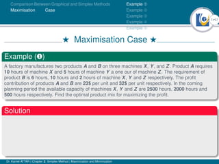
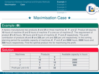
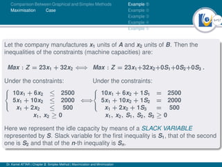
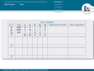
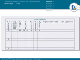
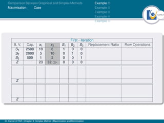
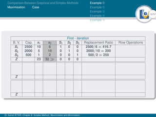
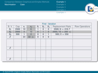
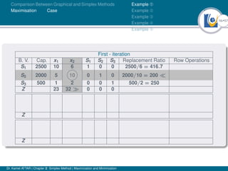
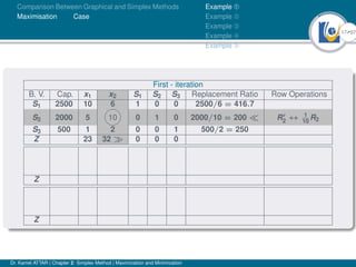
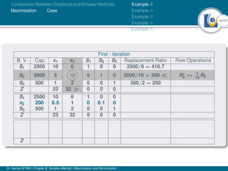
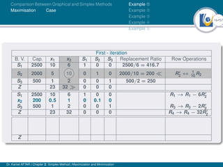
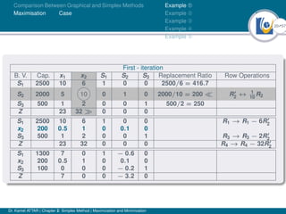
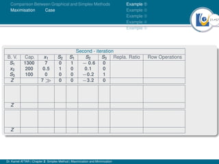
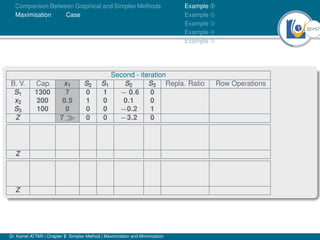
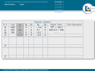
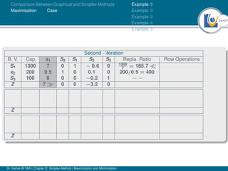
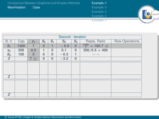
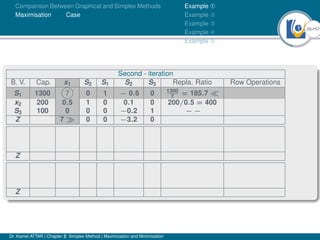
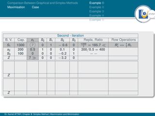
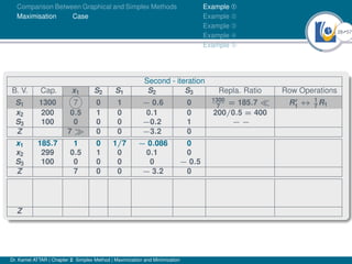
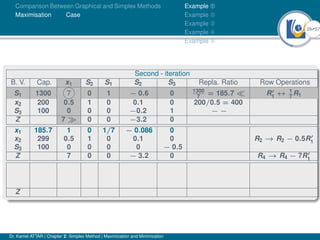
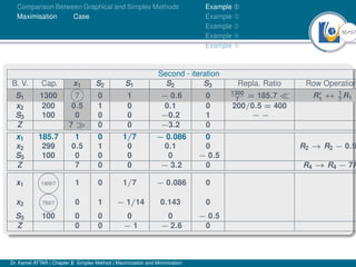
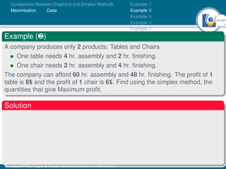
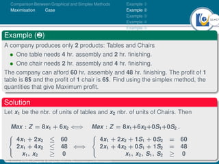
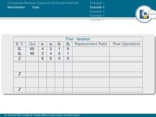
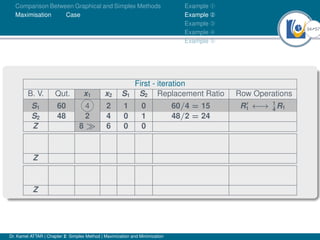
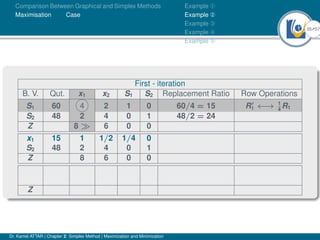
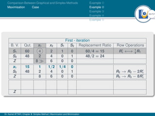
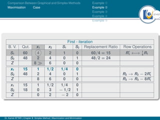
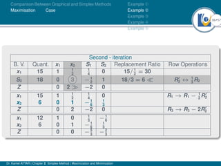
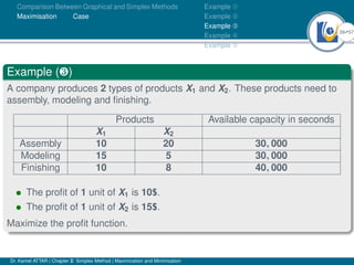
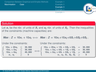
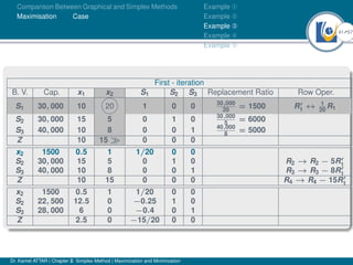
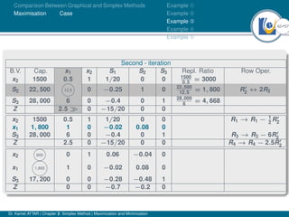
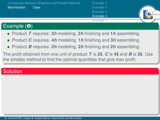
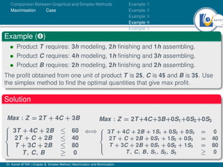
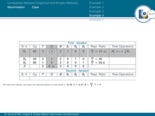
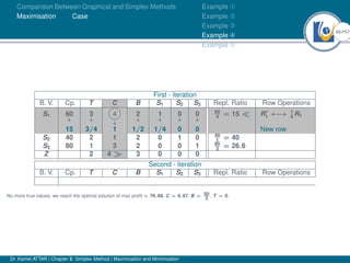
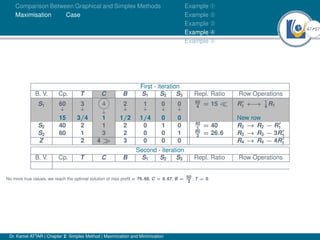
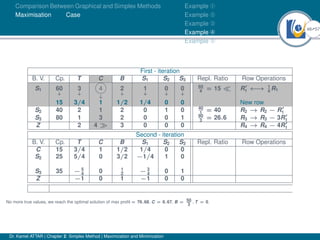
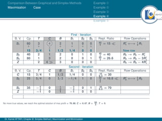
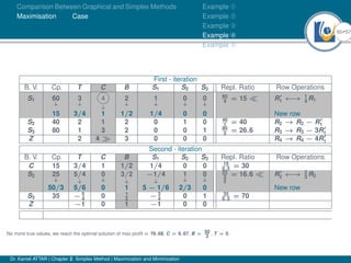
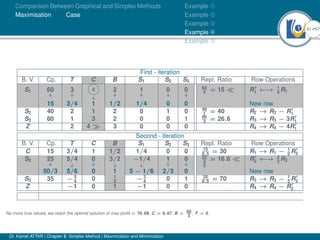
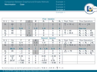
Faculty of Economics and Business Administration
Lebanese University
Chapter 2: Simplex Method
(Maximization and Minimization)
Dr. Kamel ATTAR
attar.kamel@gmail.com
Lecture #3 F Monday 8/Mar/2021 F
2Ú57
Comparison Between Graphical and Simplex Methods
Maximisation Case
1 Comparison Between Graphical and Simplex Methods
2 Maximisation Case
Example À
Example Á
Example Â
Example Ã
Example Ä
Dr. Kamel ATTAR | Chapter 2: Simplex Method | Maximization and Minimization
3Ú57
Comparison Between Graphical and Simplex Methods
Maximisation Case
H Comparison Between Graphical and Simplex Methods H
À I Graphical method is used when we have two decision variables in the
problem.
I Simplex method, is used when we have any number of decision variables.
Dr. Kamel ATTAR | Chapter 2: Simplex Method | Maximization and Minimization
4Ú57
Comparison Between Graphical and Simplex Methods
Maximisation Case
H Comparison Between Graphical and Simplex Methods H
À I Graphical method is used when we have two decision variables in the
problem.
I Simplex method, is used when we have any number of decision variables.
Á I In graphical method, the inequalities are assumed to be equations, so as to
enable to draw straight lines.
I In Simplex method, the inequalities are converted into equations by:
(i) Adding a SLACK VARIABLE in maximisation problem.
(ii) Subtracting a SURPLUS VARIABLE in case of minimization problem.
Dr. Kamel ATTAR | Chapter 2: Simplex Method | Maximization and Minimization
5Ú57
Comparison Between Graphical and Simplex Methods
Maximisation Case
H Comparison Between Graphical and Simplex Methods H
À I Graphical method is used when we have two decision variables in the
problem.
I Simplex method, is used when we have any number of decision variables.
Á I In graphical method, the inequalities are assumed to be equations, so as to
enable to draw straight lines.
I In Simplex method, the inequalities are converted into equations by:
(i) Adding a SLACK VARIABLE in maximisation problem.
(ii) Subtracting a SURPLUS VARIABLE in case of minimization problem.
 I In graphical method, the areas outside the feasible area (area covered by all
the lines of constraints in the problem) indicates idle capacity of resource
I In Simplex method, the presence of slack variable indicates the idle capacity
of the resources.
Dr. Kamel ATTAR | Chapter 2: Simplex Method | Maximization and Minimization
6Ú57
Comparison Between Graphical and Simplex Methods
Maximisation Case
H Comparison Between Graphical and Simplex Methods H
À I Graphical method is used when we have two decision variables in the
problem.
I Simplex method, is used when we have any number of decision variables.
Á I In graphical method, the inequalities are assumed to be equations, so as to
enable to draw straight lines.
I In Simplex method, the inequalities are converted into equations by:
(i) Adding a SLACK VARIABLE in maximisation problem.
(ii) Subtracting a SURPLUS VARIABLE in case of minimization problem.
 I In graphical method, the areas outside the feasible area (area covered by all
the lines of constraints in the problem) indicates idle capacity of resource
I In Simplex method, the presence of slack variable indicates the idle capacity
of the resources.
à I In graphical method, if the isoprofit line coincides with more than one point of
the feasible polygon, then the problem has second alternate solution.
I In Simplex method, the netevaluation row has zero for non-basis variable the
problem has alternate solution.
Dr. Kamel ATTAR | Chapter 2: Simplex Method | Maximization and Minimization
7Ú57
Comparison Between Graphical and Simplex Methods
Maximisation Case
Example À
Example Á
Example Â
Example Ã
Example Ä
H Maximisation Case H
Example (¶)
A factory manufactures two products A and B on three machines X, Y, and Z. Product A requires
10 hours of machine X and 5 hours of machine Y a one our of machine Z. The requirement of
product B is 6 hours, 10 hours and 2 hours of machine X, Y and Z respectively. The profit
contribution of products A and B are 23$ per unit and 32$ per unit respectively. In the coming
planning period the available capacity of machines X, Y and Z are 2500 hours, 2000 hours and
500 hours respectively. Find the optimal product mix for maximizing the profit.
Solution
Dr. Kamel ATTAR | Chapter 2: Simplex Method | Maximization and Minimization
8Ú57
Comparison Between Graphical and Simplex Methods
Maximisation Case
Example À
Example Á
Example Â
Example Ã
Example Ä
H Maximisation Case H
Example (¶)
A factory manufactures two products A and B on three machines X, Y, and Z. Product A requires
10 hours of machine X and 5 hours of machine Y a one our of machine Z. The requirement of
product B is 6 hours, 10 hours and 2 hours of machine X, Y and Z respectively. The profit
contribution of products A and B are 23$ per unit and 32$ per unit respectively. In the coming
planning period the available capacity of machines X, Y and Z are 2500 hours, 2000 hours and
500 hours respectively. Find the optimal product mix for maximizing the profit.
Solution
Machines Products Available capacity in hours
A B
X 10 6 2500
Y 5 10 2000
Z 1 2 500
Profit per unit in $ 23 32
Dr. Kamel ATTAR | Chapter 2: Simplex Method | Maximization and Minimization
9Ú57
Comparison Between Graphical and Simplex Methods
Maximisation Case
Example À
Example Á
Example Â
Example Ã
Example Ä
Let the company manufactures x1 units of A and x2 units of B. Then the
inequalities of the constraints (machine capacities) are:
Max : Z = 23x1 + 32x2 ⇐⇒
Under the constraints:



10x1 + 6x2 ≤ 2500
5x1 + 10x2 ≤ 2000
x1 + 2x2 ≤ 500
⇐⇒
x1, x2 ≥ 0
Max : Z = 23x1+32x2+0S1+0S2+0S3 .
Under the constraints:



10x1 + 6x2 + 1S1 = 2500
5x1 + 10x2 + 1S2 = 2000
x1 + 2x2 + 1S3 = 500
x1, x2, S1, S2, S3 ≥ 0
Here we represent the idle capacity by means of a SLACK VARIABLE
represented by S. Slack variable for the first inequality is S1, that of the second
one is S2 and that of the n-th inequality is Sn.
Dr. Kamel ATTAR | Chapter 2: Simplex Method | Maximization and Minimization
10Ú57
Comparison Between Graphical and Simplex Methods
Maximisation Case
Example À
Example Á
Example Â
Example Ã
Example Ä
First - iteration
B. V. Cap. x1 x2 S1 S2 S3 Replacement Ratio Row Operations
S1 2500 10 6 1 0 0
S2 2000 5 10 0 1 0
S3 500 1 2 0 0 1
Z 23 32 0 0 0
Z
Z
Dr. Kamel ATTAR | Chapter 2: Simplex Method | Maximization and Minimization
11Ú57
Comparison Between Graphical and Simplex Methods
Maximisation Case
Example À
Example Á
Example Â
Example Ã
Example Ä
First - iteration
B. V. Cap. x1 x2 S1 S2 S3 Replacement Ratio Row Operations
S1 2500 10 6 1 0 0
S2 2000 5 10 0 1 0
S3 500 1 2 0 0 1
Z 23 32  0 0 0
Z
Z
Dr. Kamel ATTAR | Chapter 2: Simplex Method | Maximization and Minimization
12Ú57
Comparison Between Graphical and Simplex Methods
Maximisation Case
Example À
Example Á
Example Â
Example Ã
Example Ä
First - iteration
B. V. Cap. x1 x2 S1 S2 S3 Replacement Ratio Row Operations
S1 2500 10 6 1 0 0
S2 2000 5 10 0 1 0
S3 500 1 2 0 0 1
Z 23 32  0 0 0
Z
Z
Dr. Kamel ATTAR | Chapter 2: Simplex Method | Maximization and Minimization
13Ú57
Comparison Between Graphical and Simplex Methods
Maximisation Case
Example À
Example Á
Example Â
Example Ã
Example Ä
First - iteration
B. V. Cap. x1 x2 S1 S2 S3 Replacement Ratio Row Operations
S1 2500 10 6 1 0 0 2500/6 = 416.7
S2 2000 5 10 0 1 0 2000/10 = 200
S3 500 1 2 0 0 1 500/2 = 250
Z 23 32  0 0 0
Z
Z
Dr. Kamel ATTAR | Chapter 2: Simplex Method | Maximization and Minimization
14Ú57
Comparison Between Graphical and Simplex Methods
Maximisation Case
Example À
Example Á
Example Â
Example Ã
Example Ä
First - iteration
B. V. Cap. x1 x2 S1 S2 S3 Replacement Ratio Row Operations
S1 2500 10 6 1 0 0 2500/6 = 416.7
S2 2000 5 10 0 1 0 2000/10 = 200 
S3 500 1 2 0 0 1 500/2 = 250
Z 23 32  0 0 0
Z
Z
Dr. Kamel ATTAR | Chapter 2: Simplex Method | Maximization and Minimization
15Ú57
Comparison Between Graphical and Simplex Methods
Maximisation Case
Example À
Example Á
Example Â
Example Ã
Example Ä
First - iteration
B. V. Cap. x1 x2 S1 S2 S3 Replacement Ratio Row Operations
S1 2500 10 6 1 0 0 2500/6 = 416.7
S2 2000 5 10 0 1 0 2000/10 = 200 
S3 500 1 2 0 0 1 500/2 = 250
Z 23 32  0 0 0
Z
Z
Dr. Kamel ATTAR | Chapter 2: Simplex Method | Maximization and Minimization
16Ú57
Comparison Between Graphical and Simplex Methods
Maximisation Case
Example À
Example Á
Example Â
Example Ã
Example Ä
First - iteration
B. V. Cap. x1 x2 S1 S2 S3 Replacement Ratio Row Operations
S1 2500 10 6 1 0 0 2500/6 = 416.7
S2 2000 5 10 0 1 0 2000/10 = 200 
S3 500 1 2 0 0 1 500/2 = 250
Z 23 32  0 0 0
Z
Z
Dr. Kamel ATTAR | Chapter 2: Simplex Method | Maximization and Minimization
17Ú57
Comparison Between Graphical and Simplex Methods
Maximisation Case
Example À
Example Á
Example Â
Example Ã
Example Ä
First - iteration
B. V. Cap. x1 x2 S1 S2 S3 Replacement Ratio Row Operations
S1 2500 10 6 1 0 0 2500/6 = 416.7
S2 2000 5 10 0 1 0 2000/10 = 200  R0
2 ↔ 1
10
R2
S3 500 1 2 0 0 1 500/2 = 250
Z 23 32  0 0 0
Z
Z
Dr. Kamel ATTAR | Chapter 2: Simplex Method | Maximization and Minimization
18Ú57
Comparison Between Graphical and Simplex Methods
Maximisation Case
Example À
Example Á
Example Â
Example Ã
Example Ä
First - iteration
B. V. Cap. x1 x2 S1 S2 S3 Replacement Ratio Row Operations
S1 2500 10 6 1 0 0 2500/6 = 416.7
S2 2000 5 10 0 1 0 2000/10 = 200  R0
2 ↔ 1
10
R2
S3 500 1 2 0 0 1 500/2 = 250
Z 23 32  0 0 0
S1 2500 10 6 1 0 0
x2 200 0.5 1 0 0.1 0
S3 500 1 2 0 0 1
Z 23 32 0 0 0
Z
Dr. Kamel ATTAR | Chapter 2: Simplex Method | Maximization and Minimization
19Ú57
Comparison Between Graphical and Simplex Methods
Maximisation Case
Example À
Example Á
Example Â
Example Ã
Example Ä
First - iteration
B. V. Cap. x1 x2 S1 S2 S3 Replacement Ratio Row Operations
S1 2500 10 6 1 0 0 2500/6 = 416.7
S2 2000 5 10 0 1 0 2000/10 = 200  R0
2 ↔ 1
10
R2
S3 500 1 2 0 0 1 500/2 = 250
Z 23 32  0 0 0
S1 2500 10 6 1 0 0 R1 → R1 − 6R0
2
x2 200 0.5 1 0 0.1 0
S3 500 1 2 0 0 1 R3 → R3 − 2R0
2
Z 23 32 0 0 0 R4 → R4 − 32R0
2
Z
Dr. Kamel ATTAR | Chapter 2: Simplex Method | Maximization and Minimization
20Ú57
Comparison Between Graphical and Simplex Methods
Maximisation Case
Example À
Example Á
Example Â
Example Ã
Example Ä
First - iteration
B. V. Cap. x1 x2 S1 S2 S3 Replacement Ratio Row Operations
S1 2500 10 6 1 0 0 2500/6 = 416.7
S2 2000 5 10 0 1 0 2000/10 = 200  R0
2 ↔ 1
10
R2
S3 500 1 2 0 0 1 500/2 = 250
Z 23 32  0 0 0
S1 2500 10 6 1 0 0 R1 → R1 − 6R0
2
x2 200 0.5 1 0 0.1 0
S3 500 1 2 0 0 1 R3 → R3 − 2R0
2
Z 23 32 0 0 0 R4 → R4 − 32R0
2
S1 1300 7 0 1 − 0.6 0
x2 200 0.5 1 0 0.1 0
S3 100 0 0 0 − 0.2 1
Z 7 0 0 − 3.2 0
Dr. Kamel ATTAR | Chapter 2: Simplex Method | Maximization and Minimization
21Ú57
Comparison Between Graphical and Simplex Methods
Maximisation Case
Example À
Example Á
Example Â
Example Ã
Example Ä
Second - iteration
B. V. Cap. x1 S2 S1 S2 S3 Repla. Ratio Row Operations
S1 1300 7 0 1 − 0.6 0
x2 200 0.5 1 0 0.1 0
S3 100 0 0 0 −0.2 1
Z 7  0 0 −3.2 0
Z
Z
Dr. Kamel ATTAR | Chapter 2: Simplex Method | Maximization and Minimization
22Ú57
Comparison Between Graphical and Simplex Methods
Maximisation Case
Example À
Example Á
Example Â
Example Ã
Example Ä
Second - iteration
B. V. Cap. x1 S2 S1 S2 S3 Repla. Ratio Row Operations
S1 1300 7 0 1 − 0.6 0
x2 200 0.5 1 0 0.1 0
S3 100 0 0 0 −0.2 1
Z 7  0 0 −3.2 0
Z
Z
Dr. Kamel ATTAR | Chapter 2: Simplex Method | Maximization and Minimization
23Ú57
Comparison Between Graphical and Simplex Methods
Maximisation Case
Example À
Example Á
Example Â
Example Ã
Example Ä
Second - iteration
B. V. Cap. x1 S2 S1 S2 S3 Repla. Ratio Row Operations
S1 1300 7 0 1 − 0.6 0 1300
7
= 185.7
x2 200 0.5 1 0 0.1 0 200/0.5 = 400
S3 100 0 0 0 −0.2 1 − −
Z 7  0 0 −3.2 0
Z
Z
Dr. Kamel ATTAR | Chapter 2: Simplex Method | Maximization and Minimization
24Ú57
Comparison Between Graphical and Simplex Methods
Maximisation Case
Example À
Example Á
Example Â
Example Ã
Example Ä
Second - iteration
B. V. Cap. x1 S2 S1 S2 S3 Repla. Ratio Row Operations
S1 1300 7 0 1 − 0.6 0 1300
7
= 185.7 
x2 200 0.5 1 0 0.1 0 200/0.5 = 400
S3 100 0 0 0 −0.2 1 − −
Z 7  0 0 −3.2 0
Z
Z
Dr. Kamel ATTAR | Chapter 2: Simplex Method | Maximization and Minimization
25Ú57
Comparison Between Graphical and Simplex Methods
Maximisation Case
Example À
Example Á
Example Â
Example Ã
Example Ä
Second - iteration
B. V. Cap. x1 S2 S1 S2 S3 Repla. Ratio Row Operations
S1 1300 7 0 1 − 0.6 0 1300
7
= 185.7 
x2 200 0.5 1 0 0.1 0 200/0.5 = 400
S3 100 0 0 0 −0.2 1 − −
Z 7  0 0 −3.2 0
Z
Z
Dr. Kamel ATTAR | Chapter 2: Simplex Method | Maximization and Minimization
26Ú57
Comparison Between Graphical and Simplex Methods
Maximisation Case
Example À
Example Á
Example Â
Example Ã
Example Ä
Second - iteration
B. V. Cap. x1 S2 S1 S2 S3 Repla. Ratio Row Operations
S1 1300 7 0 1 − 0.6 0 1300
7
= 185.7 
x2 200 0.5 1 0 0.1 0 200/0.5 = 400
S3 100 0 0 0 −0.2 1 − −
Z 7  0 0 −3.2 0
Z
Z
Dr. Kamel ATTAR | Chapter 2: Simplex Method | Maximization and Minimization
27Ú57
Comparison Between Graphical and Simplex Methods
Maximisation Case
Example À
Example Á
Example Â
Example Ã
Example Ä
Second - iteration
B. V. Cap. x1 S2 S1 S2 S3 Repla. Ratio Row Operations
S1 1300 7 0 1 − 0.6 0 1300
7
= 185.7  R0
1 ↔ 1
7
R1
x2 200 0.5 1 0 0.1 0 200/0.5 = 400
S3 100 0 0 0 −0.2 1 − −
Z 7  0 0 −3.2 0
Z
Z
Dr. Kamel ATTAR | Chapter 2: Simplex Method | Maximization and Minimization
28Ú57
Comparison Between Graphical and Simplex Methods
Maximisation Case
Example À
Example Á
Example Â
Example Ã
Example Ä
Second - iteration
B. V. Cap. x1 S2 S1 S2 S3 Repla. Ratio Row Operations
S1 1300 7 0 1 − 0.6 0 1300
7
= 185.7  R0
1 ↔ 1
7
R1
x2 200 0.5 1 0 0.1 0 200/0.5 = 400
S3 100 0 0 0 −0.2 1 − −
Z 7  0 0 −3.2 0
x1 185.7 1 0 1/7 − 0.086 0
x2 299 0.5 1 0 0.1 0
S3 100 0 0 0 0 − 0.5
Z 7 0 0 − 3.2 0
Z
Dr. Kamel ATTAR | Chapter 2: Simplex Method | Maximization and Minimization
29Ú57
Comparison Between Graphical and Simplex Methods
Maximisation Case
Example À
Example Á
Example Â
Example Ã
Example Ä
Second - iteration
B. V. Cap. x1 S2 S1 S2 S3 Repla. Ratio Row Operations
S1 1300 7 0 1 − 0.6 0 1300
7
= 185.7  R0
1 ↔ 1
7
R1
x2 200 0.5 1 0 0.1 0 200/0.5 = 400
S3 100 0 0 0 −0.2 1 − −
Z 7  0 0 −3.2 0
x1 185.7 1 0 1/7 − 0.086 0
x2 299 0.5 1 0 0.1 0 R2 → R2 − 0.5R0
1
S3 100 0 0 0 0 − 0.5
Z 7 0 0 − 3.2 0 R4 → R4 − 7R0
1
Z
Dr. Kamel ATTAR | Chapter 2: Simplex Method | Maximization and Minimization
30Ú57
Comparison Between Graphical and Simplex Methods
Maximisation Case
Example À
Example Á
Example Â
Example Ã
Example Ä
Second - iteration
B. V. Cap. x1 S2 S1 S2 S3 Repla. Ratio Row Operation
S1 1300 7 0 1 − 0.6 0 1300
7
= 185.7  R0
1 ↔ 1
7
R1
x2 200 0.5 1 0 0.1 0 200/0.5 = 400
S3 100 0 0 0 −0.2 1 − −
Z 7  0 0 −3.2 0
x1 185.7 1 0 1/7 − 0.086 0
x2 299 0.5 1 0 0.1 0 R2 → R2 − 0.5
S3 100 0 0 0 0 − 0.5
Z 7 0 0 − 3.2 0 R4 → R4 − 7R
x1 1300/7 1 0 1/7 − 0.086 0
x2 750/7 0 1 − 1/14 0.143 0
S3 100 0 0 0 0 − 0.5
Z 0 0 − 1 − 2.6 0
Dr. Kamel ATTAR | Chapter 2: Simplex Method | Maximization and Minimization
31Ú57
Comparison Between Graphical and Simplex Methods
Maximisation Case
Example À
Example Á
Example Â
Example Ã
Example Ä
Example (·)
A company produces only 2 products: Tables and Chairs
• One table needs 4 hr. assembly and 2 hr. finishing.
• One chair needs 2 hr. assembly and 4 hr. finishing.
The company can afford 60 hr. assembly and 48 hr. finishing. The profit of 1
table is 8$ and the profit of 1 chair is 6$. Find using the simplex method, the
quantities that give Maximum profit.
Solution
Dr. Kamel ATTAR | Chapter 2: Simplex Method | Maximization and Minimization
32Ú57
Comparison Between Graphical and Simplex Methods
Maximisation Case
Example À
Example Á
Example Â
Example Ã
Example Ä
Example (·)
A company produces only 2 products: Tables and Chairs
• One table needs 4 hr. assembly and 2 hr. finishing.
• One chair needs 2 hr. assembly and 4 hr. finishing.
The company can afford 60 hr. assembly and 48 hr. finishing. The profit of 1
table is 8$ and the profit of 1 chair is 6$. Find using the simplex method, the
quantities that give Maximum profit.
Solution
Let x1 be the nbr. of units of tables and x2 nbr. of units of Chairs. Then
Max : Z = 8x1 + 6x2 ⇐⇒



4x1 + 2x2 ≤ 60
2x1 + 4x2 ≤ 48
x1, x2 ≥ 0
⇐⇒
Max : Z = 8x1+6x2+0S1+0S2 .



4x1 + 2x2 + 1S1 + 0S2 = 60
2x1 + 4x2 + 0S1 + 1S2 = 48
x1, x2, S1, S2 ≥ 0
Dr. Kamel ATTAR | Chapter 2: Simplex Method | Maximization and Minimization
33Ú57
Comparison Between Graphical and Simplex Methods
Maximisation Case
Example À
Example Á
Example Â
Example Ã
Example Ä
First - iteration
B. V. Qut. x1 x2 S1 S2 Replacement Ratio Row Operations
S1 60 4 2 1 0
S2 48 2 4 0 1
Z 8 6 0 0
Z
Z
Dr. Kamel ATTAR | Chapter 2: Simplex Method | Maximization and Minimization
34Ú57
Comparison Between Graphical and Simplex Methods
Maximisation Case
Example À
Example Á
Example Â
Example Ã
Example Ä
First - iteration
B. V. Qut. x1 x2 S1 S2 Replacement Ratio Row Operations
S1 60 4 2 1 0 60/4 = 15 R0
1 ←→ 1
4
R1
S2 48 2 4 0 1 48/2 = 24
Z 8  6 0 0
Z
Z
Dr. Kamel ATTAR | Chapter 2: Simplex Method | Maximization and Minimization
35Ú57
Comparison Between Graphical and Simplex Methods
Maximisation Case
Example À
Example Á
Example Â
Example Ã
Example Ä
First - iteration
B. V. Qut. x1 x2 S1 S2 Replacement Ratio Row Operations
S1 60 4 2 1 0 60/4 = 15 R0
1 ←→ 1
4
R1
S2 48 2 4 0 1 48/2 = 24
Z 8  6 0 0
x1 15 1 1/2 1/4 0
S2 48 2 4 0 1
Z 8 6 0 0
Z
Dr. Kamel ATTAR | Chapter 2: Simplex Method | Maximization and Minimization
36Ú57
Comparison Between Graphical and Simplex Methods
Maximisation Case
Example À
Example Á
Example Â
Example Ã
Example Ä
First - iteration
B. V. Qut. x1 x2 S1 S2 Replacement Ratio Row Operations
S1 60 4 2 1 0 60/4 = 15 R0
1 ←→ 1
4
R1
S2 48 2 4 0 1 48/2 = 24
Z 8  6 0 0
x1 15 1 1/2 1/4 0
S2 48 2 4 0 1 R2 → R2 − 2R0
1
Z 8 6 0 0 R3 → R3 − 8R0
1
Z
Dr. Kamel ATTAR | Chapter 2: Simplex Method | Maximization and Minimization
37Ú57
Comparison Between Graphical and Simplex Methods
Maximisation Case
Example À
Example Á
Example Â
Example Ã
Example Ä
First - iteration
B. V. Qut. x1 x2 S1 S2 Replacement Ratio Row Operations
S1 60 4 2 1 0 60/4 = 15 R0
1 ←→ 1
4
R1
S2 48 2 4 0 1 48/2 = 24
Z 8  6 0 0
x1 15 1 1/2 1/4 0
S2 48 2 4 0 1 R2 → R2 − 2R0
1
Z 8 6 0 0 R3 → R3 − 8R0
1
x1 15 1 1/2 1/4 0
S2 18 0 3 − 1/2 1
Z 0 2 − 2 0
Dr. Kamel ATTAR | Chapter 2: Simplex Method | Maximization and Minimization
38Ú57
Comparison Between Graphical and Simplex Methods
Maximisation Case
Example À
Example Á
Example Â
Example Ã
Example Ä
Second - iteration
B. V. Quant. x1 x2 S1 S2 Replacement Ratio Row Operations
x1 15 1 1
2
1
4
0 15/1
2
= 30
S2 18 0 3 −1
2
1 18/3 = 6  R0
2 ↔ 1
3
R2
Z 0 2  −2 0
x1 15 1 1
2
1
4
0 R1 → R1 − 1
2
R0
2
x2 6 0 1 −1
6
1
3
Z 0 2 −2 0 R3 → R3 − 2R0
2
x1 12 1 0 1
3
−1
6
x2 6 0 1 −1
6
1
3
Z 0 0 −5
3
−2
3
Dr. Kamel ATTAR | Chapter 2: Simplex Method | Maximization and Minimization
39Ú57
Comparison Between Graphical and Simplex Methods
Maximisation Case
Example À
Example Á
Example Â
Example Ã
Example Ä
Example (¸)
A company produces 2 types of products X1 and X2. These products need to
assembly, modeling and finishing.
Products Available capacity in seconds
X1 X2
Assembly 10 20 30, 000
Modeling 15 5 30, 000
Finishing 10 8 40, 000
• The profit of 1 unit of X1 is 10$.
• The profit of 1 unit of X2 is 15$.
Maximize the profit function.
Dr. Kamel ATTAR | Chapter 2: Simplex Method | Maximization and Minimization
40Ú57
Comparison Between Graphical and Simplex Methods
Maximisation Case
Example À
Example Á
Example Â
Example Ã
Example Ä
Solution
Let x1 be the nbr. of units of X1 and x2 nbr. of units of X2. Then the inequalities
of the constraints (machine capacities) are:
Max : Z = 10x1 + 15x2 ⇐⇒
Under the constraints:



10x1 + 20x2 ≤ 30, 000
15x1 + 5x2 ≤ 30, 000
10x1 + 8x2 ≤ 40, 000
x1, x2 ≥ 0
⇐⇒
Max : Z = 10x1+15x2+0S1+0S2+0S3 .
Under the constraints:



10x1 + 20x2 + 1S1 + 0S2 + 0S3 = 30, 000
15x1 + 5x2 + 0S1 + 1S2 + 0S3 = 30, 000
10x1 + 8x2 + 0S1 + 0S2 + 1S3 = 40, 000
x1, x2, S1, S2, S3 ≥ 0
Dr. Kamel ATTAR | Chapter 2: Simplex Method | Maximization and Minimization
41Ú57
Comparison Between Graphical and Simplex Methods
Maximisation Case
Example À
Example Á
Example Â
Example Ã
Example Ä
First - iteration
B. V. Cap. x1 x2 S1 S2 S3 Replacement Ratio Row Oper.
S1 30, 000 10 20 1 0 0 30,000
20
= 1500 R0
1 ↔ 1
20
R1
S2 30, 000 15 5 0 1 0 30,000
5
= 6000
S3 40, 000 10 8 0 0 1 40,000
8
= 5000
Z 10 15  0 0 0
x2 1500 0.5 1 1/20 0 0
S2 30, 000 15 5 0 1 0 R2 → R2 − 5R0
1
S3 40, 000 10 8 0 0 1 R3 → R3 − 8R0
1
Z 10 15 0 0 0 R4 → R4 − 15R0
1
x2 1500 0.5 1 1/20 0 0
S2 22, 500 12.5 0 −0.25 1 0
S3 28, 000 6 0 −0.4 0 1
Z 2.5 0 −15/20 0 0
Dr. Kamel ATTAR | Chapter 2: Simplex Method | Maximization and Minimization
42Ú57
Comparison Between Graphical and Simplex Methods
Maximisation Case
Example À
Example Á
Example Â
Example Ã
Example Ä
Second - iteration
B.V. Cap. x1 x2 S1 S2 S3 Repl. Ratio Row Oper.
x2 1500 0.5 1 1/20 0 0 1500
0.5
= 3000
S2 22, 500 12.5 0 −0.25 1 0 22,500
12.5
= 1, 800 R0
2 ↔ 2R2
S3 28, 000 6 0 −0.4 0 1 28,000
6
= 4, 668
Z 2.5  0 −15/20 0 0
x2 1500 0.5 1 1/20 0 0 R1 → R1 − 1
2
R0
2
x1 1, 800 1 0 −0.02 0.08 0
S3 28, 000 6 0 −0.4 0 1 R3 → R3 − 6R0
2
Z 2.5 0 −15/20 0 0 R4 → R4 − 2.5R0
2
x2 600 0 1 0.06 −0.04 0
x1 1,800 1 0 −0.02 0.08 0
S3 17, 200 0 0 −0.28 −0.48 1
Z 0 0 −0.7 −0.2 0
Dr. Kamel ATTAR | Chapter 2: Simplex Method | Maximization and Minimization
43Ú57
Comparison Between Graphical and Simplex Methods
Maximisation Case
Example À
Example Á
Example Â
Example Ã
Example Ä
Example (¹)
• Product T requires: 3h modeling, 2h finishing and 1h assembling.
• Product C requires: 4h modeling, 1h finishing and 3h assembling.
• Product B requires: 2h modeling, 2h finishing and 2h assembling.
The profit obtained from one unit of product T is 2$, C is 4$ and B is 3$. Use
the simplex method to find the optimal quantities that give max profit.
Solution
Dr. Kamel ATTAR | Chapter 2: Simplex Method | Maximization and Minimization
44Ú57
Comparison Between Graphical and Simplex Methods
Maximisation Case
Example À
Example Á
Example Â
Example Ã
Example Ä
Example (¹)
• Product T requires: 3h modeling, 2h finishing and 1h assembling.
• Product C requires: 4h modeling, 1h finishing and 3h assembling.
• Product B requires: 2h modeling, 2h finishing and 2h assembling.
The profit obtained from one unit of product T is 2$, C is 4$ and B is 3$. Use
the simplex method to find the optimal quantities that give max profit.
Solution
Max : Z = 2T + 4C + 3B







3T + 4C + 2B ≤ 60
2T + C + 2B ≤ 40
T + 3C + 2B ≤ 80
T, C, B ≥ 0
⇐⇒
Max : Z = 2T+4C+3B+0S1+0S2+0S3





3T + 4C + 2B + 1S1 + 0S2 + 0S3 = 0
2T + C + 2B + 0S1 + 1S2 + 0S3 = 40
T + 3C + 2B + 0S1 + 0S2 + 1S3 = 80
T, C, B, S1, S2, S3 ≥ 0
Dr. Kamel ATTAR | Chapter 2: Simplex Method | Maximization and Minimization
45Ú57
Comparison Between Graphical and Simplex Methods
Maximisation Case
Example À
Example Á
Example Â
Example Ã
Example Ä
First - iteration
B. V. Cp. T C B S1 S2 S3 Repl. Ratio Row Operations
S1 60 3 4 2 1 0 0 60
4 = 15  R0
1 ←
→ 1
4 R1
S2 40 2 1 2 0 1 0 40
1 = 40
S3 80 1 3 2 0 0 1 80
3 = 26.6
Z 2 4  3 0 0 0
Second - iteration
B. V. Cp. T C B S1 S2 S3 Repl. Ratio Row Operations
No more true values, we reach the optimal solution of max profit = 76.68, C = 6.67, B = 50
3
, T = 0.
Dr. Kamel ATTAR | Chapter 2: Simplex Method | Maximization and Minimization
46Ú57
Comparison Between Graphical and Simplex Methods
Maximisation Case
Example À
Example Á
Example Â
Example Ã
Example Ä
First - iteration
B. V. Cp. T C B S1 S2 S3 Repl. Ratio Row Operations
S1 60
↓
3
↓
4
↓
2
↓
1
↓
0
↓
0
↓
60
4 = 15  R0
1 ←
→ 1
4 R1
15 3/4 1 1/2 1/4 0 0 New row
S2 40 2 1 2 0 1 0 40
1 = 40
S3 80 1 3 2 0 0 1 80
3 = 26.6
Z 2 4  3 0 0 0
Second - iteration
B. V. Cp. T C B S1 S2 S3 Repl. Ratio Row Operations
No more true values, we reach the optimal solution of max profit = 76.68, C = 6.67, B = 50
3
, T = 0.
Dr. Kamel ATTAR | Chapter 2: Simplex Method | Maximization and Minimization
47Ú57
Comparison Between Graphical and Simplex Methods
Maximisation Case
Example À
Example Á
Example Â
Example Ã
Example Ä
First - iteration
B. V. Cp. T C B S1 S2 S3 Repl. Ratio Row Operations
S1 60
↓
3
↓
4
↓
2
↓
1
↓
0
↓
0
↓
60
4 = 15  R0
1 ←
→ 1
4 R1
15 3/4 1 1/2 1/4 0 0 New row
S2 40 2 1 2 0 1 0 40
1 = 40 R2 → R2 − R0
1
S3 80 1 3 2 0 0 1 80
3 = 26.6 R3 → R3 − 3R0
1
Z 2 4  3 0 0 0 R4 → R4 − 4R0
1
Second - iteration
B. V. Cp. T C B S1 S2 S3 Repl. Ratio Row Operations
No more true values, we reach the optimal solution of max profit = 76.68, C = 6.67, B = 50
3
, T = 0.
Dr. Kamel ATTAR | Chapter 2: Simplex Method | Maximization and Minimization
48Ú57
Comparison Between Graphical and Simplex Methods
Maximisation Case
Example À
Example Á
Example Â
Example Ã
Example Ä
First - iteration
B. V. Cp. T C B S1 S2 S3 Repl. Ratio Row Operations
S1 60
↓
3
↓
4
↓
2
↓
1
↓
0
↓
0
↓
60
4 = 15  R0
1 ←
→ 1
4 R1
15 3/4 1 1/2 1/4 0 0 New row
S2 40 2 1 2 0 1 0 40
1 = 40 R2 → R2 − R0
1
S3 80 1 3 2 0 0 1 80
3 = 26.6 R3 → R3 − 3R0
1
Z 2 4  3 0 0 0 R4 → R4 − 4R0
1
Second - iteration
B. V. Cp. T C B S1 S2 S3 Repl. Ratio Row Operations
C 15 3/4 1 1/2 1/4 0 0
S2 25 5/4 0 3/2 −1/4 1 0
S3 35 − 5
4 0 1
2 − 3
4 0 1
Z −1 0 1 −1 0 0
No more true values, we reach the optimal solution of max profit = 76.68, C = 6.67, B = 50
3
, T = 0.
Dr. Kamel ATTAR | Chapter 2: Simplex Method | Maximization and Minimization
49Ú57
Comparison Between Graphical and Simplex Methods
Maximisation Case
Example À
Example Á
Example Â
Example Ã
Example Ä
First - iteration
B. V. Cp. T C B S1 S2 S3 Repl. Ratio Row Operations
S1 60
↓
3
↓
4
↓
2
↓
1
↓
0
↓
0
↓
60
4 = 15  R0
1 ←
→ 1
4 R1
15 3/4 1 1/2 1/4 0 0 New row
S2 40 2 1 2 0 1 0 40
1 = 40 R2 → R2 − R0
1
S3 80 1 3 2 0 0 1 80
3 = 26.6 R3 → R3 − 3R0
1
Z 2 4  3 0 0 0 R4 → R4 − 4R0
1
Second - iteration
B. V. Cp. T C B S1 S2 S3 Repl. Ratio Row Operations
C 15 3/4 1 1/2 1/4 0 0 15
0.5 = 30
S2 25 5/4 0 3/2 −1/4 1 0 25
3
2
= 16.6  R0
2 ←
→ 2
3 R2
S3 35 − 5
4 0 1
2 − 3
4 0 1 35
0.5 = 70
Z −1 0 1 −1 0 0
No more true values, we reach the optimal solution of max profit = 76.68, C = 6.67, B = 50
3
, T = 0.
Dr. Kamel ATTAR | Chapter 2: Simplex Method | Maximization and Minimization
50Ú57
Comparison Between Graphical and Simplex Methods
Maximisation Case
Example À
Example Á
Example Â
Example Ã
Example Ä
First - iteration
B. V. Cp. T C B S1 S2 S3 Repl. Ratio Row Operations
S1 60
↓
3
↓
4
↓
2
↓
1
↓
0
↓
0
↓
60
4 = 15  R0
1 ←
→ 1
4 R1
15 3/4 1 1/2 1/4 0 0 New row
S2 40 2 1 2 0 1 0 40
1 = 40 R2 → R2 − R0
1
S3 80 1 3 2 0 0 1 80
3 = 26.6 R3 → R3 − 3R0
1
Z 2 4  3 0 0 0 R4 → R4 − 4R0
1
Second - iteration
B. V. Cp. T C B S1 S2 S3 Repl. Ratio Row Operations
C 15 3/4 1 1/2 1/4 0 0 15
0.5 = 30
S2 25
↓
5/4
↓
0
↓
3/2
↓
−1/4
↓
1
↓
0
↓
25
3
2
= 16.6  R0
2 ←
→ 2
3 R2
50/3 5/6 0 1 5 − 1/6 2/3 0 New row
S3 35 − 5
4 0 1
2 − 3
4 0 1 35
0.5 = 70
Z −1 0 1 −1 0 0
No more true values, we reach the optimal solution of max profit = 76.68, C = 6.67, B = 50
3
, T = 0.
Dr. Kamel ATTAR | Chapter 2: Simplex Method | Maximization and Minimization
51Ú57
Comparison Between Graphical and Simplex Methods
Maximisation Case
Example À
Example Á
Example Â
Example Ã
Example Ä
First - iteration
B. V. Cp. T C B S1 S2 S3 Repl. Ratio Row Operations
S1 60
↓
3
↓
4
↓
2
↓
1
↓
0
↓
0
↓
60
4 = 15  R0
1 ←
→ 1
4 R1
15 3/4 1 1/2 1/4 0 0 New row
S2 40 2 1 2 0 1 0 40
1 = 40 R2 → R2 − R0
1
S3 80 1 3 2 0 0 1 80
3 = 26.6 R3 → R3 − 3R0
1
Z 2 4  3 0 0 0 R4 → R4 − 4R0
1
Second - iteration
B. V. Cp. T C B S1 S2 S3 Repl. Ratio Row Operations
C 15 3/4 1 1/2 1/4 0 0 15
0.5 = 30 R1 → R1 − 1
2 R0
2
S2 25
↓
5/4
↓
0
↓
3/2
↓
−1/4
↓
1
↓
0
↓
25
3
2
= 16.6  R0
2 ←
→ 2
3 R2
50/3 5/6 0 1 5 − 1/6 2/3 0 New row
S3 35 − 5
4 0 1
2 − 3
4 0 1 35
0.5 = 70 R3 → R3 − 1
2 R0
2
Z −1 0 1 −1 0 0 R4 → R4 − R0
2
No more true values, we reach the optimal solution of max profit = 76.68, C = 6.67, B = 50
3
, T = 0.
Dr. Kamel ATTAR | Chapter 2: Simplex Method | Maximization and Minimization
52Ú57
Comparison Between Graphical and Simplex Methods
Maximisation Case
Example À
Example Á
Example Â
Example Ã
Example Ä
First - iteration
B. V. Cp. T C B S1 S2 S3 Repl. Ratio Row Operations
S1 60
↓
3
↓
4
↓
2
↓
1
↓
0
↓
0
↓
60
4 = 15  R0
1 ←
→ 1
4 R1
15 3/4 1 1/2 1/4 0 0 New row
S2 40 2 1 2 0 1 0 40
1 = 40 R2 → R2 − R0
1
S3 80 1 3 2 0 0 1 80
3 = 26.6 R3 → R3 − 3R0
1
Z 2 4  3 0 0 0 R4 → R4 − 4R0
1
Second - iteration
B. V. Cp. T C B S1 S2 S3 Repl. Ratio Row Operations
C 15 3/4 1 1/2 1/4 0 0 15
0.5 = 30 R1 → R1 − 1
2 R0
2
S2 25
↓
5/4
↓
0
↓
3/2
↓
−1/4
↓
1
↓
0
↓
25
3
2
= 16.6  R0
2 ←
→ 2
3 R2
50/3 5/6 0 1 5 − 1/6 2/3 0 New row
S3 35 − 5
4 0 1
2 − 3
4 0 1 35
0.5 = 70 R3 → R3 − 1
2 R0
2
Z −1 0 1 −1 0 0 R4 → R4 − R0
2
C 6.67 0.33 1 0 0.33 −0.33 0
B 50
3
5
6 0 1 − 1
6
2
3 0
S3 26.67 −1.665 0 0 −0.617 0.33 1
Z −1.83 0 0 −0.82 −0.66 0
No more true values, we reach the optimal solution of max profit = 76.68, C = 6.67, B = 50
3
, T = 0.
Dr. Kamel ATTAR | Chapter 2: Simplex Method | Maximization and Minimization
53Ú57
Comparison Between Graphical and Simplex Methods
Maximisation Case
Example À
Example Á
Example Â
Example Ã
Example Ä
Example (Ä)
A company manufactures three products: X, Y and Z by using three resources.
• Each unit of product X takes three man hours and 10 hours of machine capacity and 1 cubic
meter of storage place.
• Similarly, one unit of product Y takes 5 man-hours and 2 machine hours on 1 cubic meter of
storage place
• and that of each unit of products Z is 5 man-hours, 6 machine hours and 1 cubic meter of
storage place.
The profit contribution of products X, Y and Z are 4$, 5$ and 6$ respectively. The maximum hours
of man and machine capacity are 900 and 1400 respectively and the maximum cubic meter of
storage place is 250. Use the simplex method to find the optimal solutions.
Dr. Kamel ATTAR | Chapter 2: Simplex Method | Maximization and Minimization
54Ú57
Comparison Between Graphical and Simplex Methods
Maximisation Case
Example À
Example Á
Example Â
Example Ã
Example Ä
Example (Ä)
A company manufactures three products: X, Y and Z by using three resources.
• Each unit of product X takes three man hours and 10 hours of machine capacity and 1 cubic
meter of storage place.
• Similarly, one unit of product Y takes 5 man-hours and 2 machine hours on 1 cubic meter of
storage place
• and that of each unit of products Z is 5 man-hours, 6 machine hours and 1 cubic meter of
storage place.
The profit contribution of products X, Y and Z are 4$, 5$ and 6$ respectively. The maximum hours
of man and machine capacity are 900 and 1400 respectively and the maximum cubic meter of
storage place is 250. Use the simplex method to find the optimal solutions.
solution
The linear programming is
Maximize Z = 4x1 + 5x2 + 6x3
3x1 + 5x2 + 5x3 ≤ 900
10x1 + 2x2 + 6x3 ≤ 1400
x1 + x2 + x3 ≤ 250
x1, x2, x3 ≥ 0
Dr. Kamel ATTAR | Chapter 2: Simplex Method | Maximization and Minimization
55Ú57
Comparison Between Graphical and Simplex Methods
Maximisation Case
Example À
Example Á
Example Â
Example Ã
Example Ä
solution
The problem is converted to canonical form by adding slack variables as appropiate
1. As the constraint-1 is of type ≤ we should add slack variable S1.
2. As the constraint-2 is of type ≤ we should add slack variable S2.
3. As the constraint-3 is of type ≤ we should add slack variable S3.
After introducing slack variables. The standard form The standard form
Max : Z = 4x1 + 5x2 + 6x3 + 0S1 + 0S2 + 0S3
Subject to 






3x1 + 5x2 + 5x3 + 1S1 + 0S2 + 0S3 = 900
10x1 + 2x2 + 6x3 + 0S1 + 1S2 + 0S3 = 1400
x1 + x2 + x3 + 0S1 + 0S2 + 1S3 = 250
x1, x2, x3 ≥ 0
Dr. Kamel ATTAR | Chapter 2: Simplex Method | Maximization and Minimization
56Ú57
Comparison Between Graphical and Simplex Methods
Maximisation Case
Example À
Example Á
Example Â
Example Ã
Example Ä
First - iteration
B. V. Cp. x1 x2 x3 S1 S2 S3 Min.Ratio Row Operations
S1 900
↓
3
↓
5
↓
5
↓
1
↓
0
↓
0
↓
900
5 = 180  R0
1 ←
→ 1
5 R1
180 3/5 1 1 1/5 0 0 New Row
S2 1400 10 2 6 0 1 0 1400
6 = 233.33 R2 → R2 − 6R0
1
S3 250 1 1 1 0 0 1 250
1 = 250 R3 → R3 − R0
1
Z 4 5 6  0 0 0 R4 → R4 − 6R0
1
Second - iteration
B. V. Cp. x1 x2 x3 S1 S2 S3 Min.Ratio Row Operations
x3 180 3/5 1 1 1/5 0 0 180
0.6 = 300 R1 → R1 − 3
5 R0
2
S2 320
↓
32/5
↓
−4
↓
0
↓
−6/5
↓
1
↓
0
↓
320
6.4 = 50  R0
2 ←
→ 5
32 R2
50 1 −5/8 0 −3/16 5/32 0 New Row
S3 70 2/5 0 0 −1/5 0 1 70
0.4 = 175 R3 → R3 − 2
5 R0
2
Z 2/5 −1 0 −6/5 0 0 R4 → R4 − 2
5 R0
2
x3 150 0 11/8 1 5/6 −3/32 0
x1 50 1 −5/8 0 −3/16 5/32 0
S3 50 0 1/4 0 −1/8 −1/16 1
Z 0 −23/4 0 −9/8 −1/16 0
footnotesize The solution is x1 = 50, x2 = 0, x3 = 150, S1 = 0, S2 = 0, S3 = 50 and profit Z = 1100$.
Dr. Kamel ATTAR | Chapter 2: Simplex Method | Maximization and Minimization
Thank you! Questions?

Simplex method (maximization)

  • 1.
    Faculty of Economicsand Business Administration Lebanese University Chapter 2: Simplex Method (Maximization and Minimization) Dr. Kamel ATTAR attar.kamel@gmail.com Lecture #3 F Monday 8/Mar/2021 F
  • 2.
    2Ú57 Comparison Between Graphicaland Simplex Methods Maximisation Case 1 Comparison Between Graphical and Simplex Methods 2 Maximisation Case Example À Example Á Example  Example à Example Ä Dr. Kamel ATTAR | Chapter 2: Simplex Method | Maximization and Minimization
  • 3.
    3Ú57 Comparison Between Graphicaland Simplex Methods Maximisation Case H Comparison Between Graphical and Simplex Methods H À I Graphical method is used when we have two decision variables in the problem. I Simplex method, is used when we have any number of decision variables. Dr. Kamel ATTAR | Chapter 2: Simplex Method | Maximization and Minimization
  • 4.
    4Ú57 Comparison Between Graphicaland Simplex Methods Maximisation Case H Comparison Between Graphical and Simplex Methods H À I Graphical method is used when we have two decision variables in the problem. I Simplex method, is used when we have any number of decision variables. Á I In graphical method, the inequalities are assumed to be equations, so as to enable to draw straight lines. I In Simplex method, the inequalities are converted into equations by: (i) Adding a SLACK VARIABLE in maximisation problem. (ii) Subtracting a SURPLUS VARIABLE in case of minimization problem. Dr. Kamel ATTAR | Chapter 2: Simplex Method | Maximization and Minimization
  • 5.
    5Ú57 Comparison Between Graphicaland Simplex Methods Maximisation Case H Comparison Between Graphical and Simplex Methods H À I Graphical method is used when we have two decision variables in the problem. I Simplex method, is used when we have any number of decision variables. Á I In graphical method, the inequalities are assumed to be equations, so as to enable to draw straight lines. I In Simplex method, the inequalities are converted into equations by: (i) Adding a SLACK VARIABLE in maximisation problem. (ii) Subtracting a SURPLUS VARIABLE in case of minimization problem. Â I In graphical method, the areas outside the feasible area (area covered by all the lines of constraints in the problem) indicates idle capacity of resource I In Simplex method, the presence of slack variable indicates the idle capacity of the resources. Dr. Kamel ATTAR | Chapter 2: Simplex Method | Maximization and Minimization
  • 6.
    6Ú57 Comparison Between Graphicaland Simplex Methods Maximisation Case H Comparison Between Graphical and Simplex Methods H À I Graphical method is used when we have two decision variables in the problem. I Simplex method, is used when we have any number of decision variables. Á I In graphical method, the inequalities are assumed to be equations, so as to enable to draw straight lines. I In Simplex method, the inequalities are converted into equations by: (i) Adding a SLACK VARIABLE in maximisation problem. (ii) Subtracting a SURPLUS VARIABLE in case of minimization problem. Â I In graphical method, the areas outside the feasible area (area covered by all the lines of constraints in the problem) indicates idle capacity of resource I In Simplex method, the presence of slack variable indicates the idle capacity of the resources. Ã I In graphical method, if the isoprofit line coincides with more than one point of the feasible polygon, then the problem has second alternate solution. I In Simplex method, the netevaluation row has zero for non-basis variable the problem has alternate solution. Dr. Kamel ATTAR | Chapter 2: Simplex Method | Maximization and Minimization
  • 7.
    7Ú57 Comparison Between Graphicaland Simplex Methods Maximisation Case Example À Example Á Example  Example à Example Ä H Maximisation Case H Example (¶) A factory manufactures two products A and B on three machines X, Y, and Z. Product A requires 10 hours of machine X and 5 hours of machine Y a one our of machine Z. The requirement of product B is 6 hours, 10 hours and 2 hours of machine X, Y and Z respectively. The profit contribution of products A and B are 23$ per unit and 32$ per unit respectively. In the coming planning period the available capacity of machines X, Y and Z are 2500 hours, 2000 hours and 500 hours respectively. Find the optimal product mix for maximizing the profit. Solution Dr. Kamel ATTAR | Chapter 2: Simplex Method | Maximization and Minimization
  • 8.
    8Ú57 Comparison Between Graphicaland Simplex Methods Maximisation Case Example À Example Á Example  Example à Example Ä H Maximisation Case H Example (¶) A factory manufactures two products A and B on three machines X, Y, and Z. Product A requires 10 hours of machine X and 5 hours of machine Y a one our of machine Z. The requirement of product B is 6 hours, 10 hours and 2 hours of machine X, Y and Z respectively. The profit contribution of products A and B are 23$ per unit and 32$ per unit respectively. In the coming planning period the available capacity of machines X, Y and Z are 2500 hours, 2000 hours and 500 hours respectively. Find the optimal product mix for maximizing the profit. Solution Machines Products Available capacity in hours A B X 10 6 2500 Y 5 10 2000 Z 1 2 500 Profit per unit in $ 23 32 Dr. Kamel ATTAR | Chapter 2: Simplex Method | Maximization and Minimization
  • 9.
    9Ú57 Comparison Between Graphicaland Simplex Methods Maximisation Case Example À Example Á Example  Example à Example Ä Let the company manufactures x1 units of A and x2 units of B. Then the inequalities of the constraints (machine capacities) are: Max : Z = 23x1 + 32x2 ⇐⇒ Under the constraints:    10x1 + 6x2 ≤ 2500 5x1 + 10x2 ≤ 2000 x1 + 2x2 ≤ 500 ⇐⇒ x1, x2 ≥ 0 Max : Z = 23x1+32x2+0S1+0S2+0S3 . Under the constraints:    10x1 + 6x2 + 1S1 = 2500 5x1 + 10x2 + 1S2 = 2000 x1 + 2x2 + 1S3 = 500 x1, x2, S1, S2, S3 ≥ 0 Here we represent the idle capacity by means of a SLACK VARIABLE represented by S. Slack variable for the first inequality is S1, that of the second one is S2 and that of the n-th inequality is Sn. Dr. Kamel ATTAR | Chapter 2: Simplex Method | Maximization and Minimization
  • 10.
    10Ú57 Comparison Between Graphicaland Simplex Methods Maximisation Case Example À Example Á Example  Example à Example Ä First - iteration B. V. Cap. x1 x2 S1 S2 S3 Replacement Ratio Row Operations S1 2500 10 6 1 0 0 S2 2000 5 10 0 1 0 S3 500 1 2 0 0 1 Z 23 32 0 0 0 Z Z Dr. Kamel ATTAR | Chapter 2: Simplex Method | Maximization and Minimization
  • 11.
    11Ú57 Comparison Between Graphicaland Simplex Methods Maximisation Case Example À Example Á Example  Example à Example Ä First - iteration B. V. Cap. x1 x2 S1 S2 S3 Replacement Ratio Row Operations S1 2500 10 6 1 0 0 S2 2000 5 10 0 1 0 S3 500 1 2 0 0 1 Z 23 32 0 0 0 Z Z Dr. Kamel ATTAR | Chapter 2: Simplex Method | Maximization and Minimization
  • 12.
    12Ú57 Comparison Between Graphicaland Simplex Methods Maximisation Case Example À Example Á Example  Example à Example Ä First - iteration B. V. Cap. x1 x2 S1 S2 S3 Replacement Ratio Row Operations S1 2500 10 6 1 0 0 S2 2000 5 10 0 1 0 S3 500 1 2 0 0 1 Z 23 32 0 0 0 Z Z Dr. Kamel ATTAR | Chapter 2: Simplex Method | Maximization and Minimization
  • 13.
    13Ú57 Comparison Between Graphicaland Simplex Methods Maximisation Case Example À Example Á Example  Example à Example Ä First - iteration B. V. Cap. x1 x2 S1 S2 S3 Replacement Ratio Row Operations S1 2500 10 6 1 0 0 2500/6 = 416.7 S2 2000 5 10 0 1 0 2000/10 = 200 S3 500 1 2 0 0 1 500/2 = 250 Z 23 32 0 0 0 Z Z Dr. Kamel ATTAR | Chapter 2: Simplex Method | Maximization and Minimization
  • 14.
    14Ú57 Comparison Between Graphicaland Simplex Methods Maximisation Case Example À Example Á Example  Example à Example Ä First - iteration B. V. Cap. x1 x2 S1 S2 S3 Replacement Ratio Row Operations S1 2500 10 6 1 0 0 2500/6 = 416.7 S2 2000 5 10 0 1 0 2000/10 = 200 S3 500 1 2 0 0 1 500/2 = 250 Z 23 32 0 0 0 Z Z Dr. Kamel ATTAR | Chapter 2: Simplex Method | Maximization and Minimization
  • 15.
    15Ú57 Comparison Between Graphicaland Simplex Methods Maximisation Case Example À Example Á Example  Example à Example Ä First - iteration B. V. Cap. x1 x2 S1 S2 S3 Replacement Ratio Row Operations S1 2500 10 6 1 0 0 2500/6 = 416.7 S2 2000 5 10 0 1 0 2000/10 = 200 S3 500 1 2 0 0 1 500/2 = 250 Z 23 32 0 0 0 Z Z Dr. Kamel ATTAR | Chapter 2: Simplex Method | Maximization and Minimization
  • 16.
    16Ú57 Comparison Between Graphicaland Simplex Methods Maximisation Case Example À Example Á Example  Example à Example Ä First - iteration B. V. Cap. x1 x2 S1 S2 S3 Replacement Ratio Row Operations S1 2500 10 6 1 0 0 2500/6 = 416.7 S2 2000 5 10 0 1 0 2000/10 = 200 S3 500 1 2 0 0 1 500/2 = 250 Z 23 32 0 0 0 Z Z Dr. Kamel ATTAR | Chapter 2: Simplex Method | Maximization and Minimization
  • 17.
    17Ú57 Comparison Between Graphicaland Simplex Methods Maximisation Case Example À Example Á Example  Example à Example Ä First - iteration B. V. Cap. x1 x2 S1 S2 S3 Replacement Ratio Row Operations S1 2500 10 6 1 0 0 2500/6 = 416.7 S2 2000 5 10 0 1 0 2000/10 = 200 R0 2 ↔ 1 10 R2 S3 500 1 2 0 0 1 500/2 = 250 Z 23 32 0 0 0 Z Z Dr. Kamel ATTAR | Chapter 2: Simplex Method | Maximization and Minimization
  • 18.
    18Ú57 Comparison Between Graphicaland Simplex Methods Maximisation Case Example À Example Á Example  Example à Example Ä First - iteration B. V. Cap. x1 x2 S1 S2 S3 Replacement Ratio Row Operations S1 2500 10 6 1 0 0 2500/6 = 416.7 S2 2000 5 10 0 1 0 2000/10 = 200 R0 2 ↔ 1 10 R2 S3 500 1 2 0 0 1 500/2 = 250 Z 23 32 0 0 0 S1 2500 10 6 1 0 0 x2 200 0.5 1 0 0.1 0 S3 500 1 2 0 0 1 Z 23 32 0 0 0 Z Dr. Kamel ATTAR | Chapter 2: Simplex Method | Maximization and Minimization
  • 19.
    19Ú57 Comparison Between Graphicaland Simplex Methods Maximisation Case Example À Example Á Example  Example à Example Ä First - iteration B. V. Cap. x1 x2 S1 S2 S3 Replacement Ratio Row Operations S1 2500 10 6 1 0 0 2500/6 = 416.7 S2 2000 5 10 0 1 0 2000/10 = 200 R0 2 ↔ 1 10 R2 S3 500 1 2 0 0 1 500/2 = 250 Z 23 32 0 0 0 S1 2500 10 6 1 0 0 R1 → R1 − 6R0 2 x2 200 0.5 1 0 0.1 0 S3 500 1 2 0 0 1 R3 → R3 − 2R0 2 Z 23 32 0 0 0 R4 → R4 − 32R0 2 Z Dr. Kamel ATTAR | Chapter 2: Simplex Method | Maximization and Minimization
  • 20.
    20Ú57 Comparison Between Graphicaland Simplex Methods Maximisation Case Example À Example Á Example  Example à Example Ä First - iteration B. V. Cap. x1 x2 S1 S2 S3 Replacement Ratio Row Operations S1 2500 10 6 1 0 0 2500/6 = 416.7 S2 2000 5 10 0 1 0 2000/10 = 200 R0 2 ↔ 1 10 R2 S3 500 1 2 0 0 1 500/2 = 250 Z 23 32 0 0 0 S1 2500 10 6 1 0 0 R1 → R1 − 6R0 2 x2 200 0.5 1 0 0.1 0 S3 500 1 2 0 0 1 R3 → R3 − 2R0 2 Z 23 32 0 0 0 R4 → R4 − 32R0 2 S1 1300 7 0 1 − 0.6 0 x2 200 0.5 1 0 0.1 0 S3 100 0 0 0 − 0.2 1 Z 7 0 0 − 3.2 0 Dr. Kamel ATTAR | Chapter 2: Simplex Method | Maximization and Minimization
  • 21.
    21Ú57 Comparison Between Graphicaland Simplex Methods Maximisation Case Example À Example Á Example  Example à Example Ä Second - iteration B. V. Cap. x1 S2 S1 S2 S3 Repla. Ratio Row Operations S1 1300 7 0 1 − 0.6 0 x2 200 0.5 1 0 0.1 0 S3 100 0 0 0 −0.2 1 Z 7 0 0 −3.2 0 Z Z Dr. Kamel ATTAR | Chapter 2: Simplex Method | Maximization and Minimization
  • 22.
    22Ú57 Comparison Between Graphicaland Simplex Methods Maximisation Case Example À Example Á Example  Example à Example Ä Second - iteration B. V. Cap. x1 S2 S1 S2 S3 Repla. Ratio Row Operations S1 1300 7 0 1 − 0.6 0 x2 200 0.5 1 0 0.1 0 S3 100 0 0 0 −0.2 1 Z 7 0 0 −3.2 0 Z Z Dr. Kamel ATTAR | Chapter 2: Simplex Method | Maximization and Minimization
  • 23.
    23Ú57 Comparison Between Graphicaland Simplex Methods Maximisation Case Example À Example Á Example  Example à Example Ä Second - iteration B. V. Cap. x1 S2 S1 S2 S3 Repla. Ratio Row Operations S1 1300 7 0 1 − 0.6 0 1300 7 = 185.7 x2 200 0.5 1 0 0.1 0 200/0.5 = 400 S3 100 0 0 0 −0.2 1 − − Z 7 0 0 −3.2 0 Z Z Dr. Kamel ATTAR | Chapter 2: Simplex Method | Maximization and Minimization
  • 24.
    24Ú57 Comparison Between Graphicaland Simplex Methods Maximisation Case Example À Example Á Example  Example à Example Ä Second - iteration B. V. Cap. x1 S2 S1 S2 S3 Repla. Ratio Row Operations S1 1300 7 0 1 − 0.6 0 1300 7 = 185.7 x2 200 0.5 1 0 0.1 0 200/0.5 = 400 S3 100 0 0 0 −0.2 1 − − Z 7 0 0 −3.2 0 Z Z Dr. Kamel ATTAR | Chapter 2: Simplex Method | Maximization and Minimization
  • 25.
    25Ú57 Comparison Between Graphicaland Simplex Methods Maximisation Case Example À Example Á Example  Example à Example Ä Second - iteration B. V. Cap. x1 S2 S1 S2 S3 Repla. Ratio Row Operations S1 1300 7 0 1 − 0.6 0 1300 7 = 185.7 x2 200 0.5 1 0 0.1 0 200/0.5 = 400 S3 100 0 0 0 −0.2 1 − − Z 7 0 0 −3.2 0 Z Z Dr. Kamel ATTAR | Chapter 2: Simplex Method | Maximization and Minimization
  • 26.
    26Ú57 Comparison Between Graphicaland Simplex Methods Maximisation Case Example À Example Á Example  Example à Example Ä Second - iteration B. V. Cap. x1 S2 S1 S2 S3 Repla. Ratio Row Operations S1 1300 7 0 1 − 0.6 0 1300 7 = 185.7 x2 200 0.5 1 0 0.1 0 200/0.5 = 400 S3 100 0 0 0 −0.2 1 − − Z 7 0 0 −3.2 0 Z Z Dr. Kamel ATTAR | Chapter 2: Simplex Method | Maximization and Minimization
  • 27.
    27Ú57 Comparison Between Graphicaland Simplex Methods Maximisation Case Example À Example Á Example  Example à Example Ä Second - iteration B. V. Cap. x1 S2 S1 S2 S3 Repla. Ratio Row Operations S1 1300 7 0 1 − 0.6 0 1300 7 = 185.7 R0 1 ↔ 1 7 R1 x2 200 0.5 1 0 0.1 0 200/0.5 = 400 S3 100 0 0 0 −0.2 1 − − Z 7 0 0 −3.2 0 Z Z Dr. Kamel ATTAR | Chapter 2: Simplex Method | Maximization and Minimization
  • 28.
    28Ú57 Comparison Between Graphicaland Simplex Methods Maximisation Case Example À Example Á Example  Example à Example Ä Second - iteration B. V. Cap. x1 S2 S1 S2 S3 Repla. Ratio Row Operations S1 1300 7 0 1 − 0.6 0 1300 7 = 185.7 R0 1 ↔ 1 7 R1 x2 200 0.5 1 0 0.1 0 200/0.5 = 400 S3 100 0 0 0 −0.2 1 − − Z 7 0 0 −3.2 0 x1 185.7 1 0 1/7 − 0.086 0 x2 299 0.5 1 0 0.1 0 S3 100 0 0 0 0 − 0.5 Z 7 0 0 − 3.2 0 Z Dr. Kamel ATTAR | Chapter 2: Simplex Method | Maximization and Minimization
  • 29.
    29Ú57 Comparison Between Graphicaland Simplex Methods Maximisation Case Example À Example Á Example  Example à Example Ä Second - iteration B. V. Cap. x1 S2 S1 S2 S3 Repla. Ratio Row Operations S1 1300 7 0 1 − 0.6 0 1300 7 = 185.7 R0 1 ↔ 1 7 R1 x2 200 0.5 1 0 0.1 0 200/0.5 = 400 S3 100 0 0 0 −0.2 1 − − Z 7 0 0 −3.2 0 x1 185.7 1 0 1/7 − 0.086 0 x2 299 0.5 1 0 0.1 0 R2 → R2 − 0.5R0 1 S3 100 0 0 0 0 − 0.5 Z 7 0 0 − 3.2 0 R4 → R4 − 7R0 1 Z Dr. Kamel ATTAR | Chapter 2: Simplex Method | Maximization and Minimization
  • 30.
    30Ú57 Comparison Between Graphicaland Simplex Methods Maximisation Case Example À Example Á Example  Example à Example Ä Second - iteration B. V. Cap. x1 S2 S1 S2 S3 Repla. Ratio Row Operation S1 1300 7 0 1 − 0.6 0 1300 7 = 185.7 R0 1 ↔ 1 7 R1 x2 200 0.5 1 0 0.1 0 200/0.5 = 400 S3 100 0 0 0 −0.2 1 − − Z 7 0 0 −3.2 0 x1 185.7 1 0 1/7 − 0.086 0 x2 299 0.5 1 0 0.1 0 R2 → R2 − 0.5 S3 100 0 0 0 0 − 0.5 Z 7 0 0 − 3.2 0 R4 → R4 − 7R x1 1300/7 1 0 1/7 − 0.086 0 x2 750/7 0 1 − 1/14 0.143 0 S3 100 0 0 0 0 − 0.5 Z 0 0 − 1 − 2.6 0 Dr. Kamel ATTAR | Chapter 2: Simplex Method | Maximization and Minimization
  • 31.
    31Ú57 Comparison Between Graphicaland Simplex Methods Maximisation Case Example À Example Á Example  Example à Example Ä Example (·) A company produces only 2 products: Tables and Chairs • One table needs 4 hr. assembly and 2 hr. finishing. • One chair needs 2 hr. assembly and 4 hr. finishing. The company can afford 60 hr. assembly and 48 hr. finishing. The profit of 1 table is 8$ and the profit of 1 chair is 6$. Find using the simplex method, the quantities that give Maximum profit. Solution Dr. Kamel ATTAR | Chapter 2: Simplex Method | Maximization and Minimization
  • 32.
    32Ú57 Comparison Between Graphicaland Simplex Methods Maximisation Case Example À Example Á Example  Example à Example Ä Example (·) A company produces only 2 products: Tables and Chairs • One table needs 4 hr. assembly and 2 hr. finishing. • One chair needs 2 hr. assembly and 4 hr. finishing. The company can afford 60 hr. assembly and 48 hr. finishing. The profit of 1 table is 8$ and the profit of 1 chair is 6$. Find using the simplex method, the quantities that give Maximum profit. Solution Let x1 be the nbr. of units of tables and x2 nbr. of units of Chairs. Then Max : Z = 8x1 + 6x2 ⇐⇒    4x1 + 2x2 ≤ 60 2x1 + 4x2 ≤ 48 x1, x2 ≥ 0 ⇐⇒ Max : Z = 8x1+6x2+0S1+0S2 .    4x1 + 2x2 + 1S1 + 0S2 = 60 2x1 + 4x2 + 0S1 + 1S2 = 48 x1, x2, S1, S2 ≥ 0 Dr. Kamel ATTAR | Chapter 2: Simplex Method | Maximization and Minimization
  • 33.
    33Ú57 Comparison Between Graphicaland Simplex Methods Maximisation Case Example À Example Á Example  Example à Example Ä First - iteration B. V. Qut. x1 x2 S1 S2 Replacement Ratio Row Operations S1 60 4 2 1 0 S2 48 2 4 0 1 Z 8 6 0 0 Z Z Dr. Kamel ATTAR | Chapter 2: Simplex Method | Maximization and Minimization
  • 34.
    34Ú57 Comparison Between Graphicaland Simplex Methods Maximisation Case Example À Example Á Example  Example à Example Ä First - iteration B. V. Qut. x1 x2 S1 S2 Replacement Ratio Row Operations S1 60 4 2 1 0 60/4 = 15 R0 1 ←→ 1 4 R1 S2 48 2 4 0 1 48/2 = 24 Z 8 6 0 0 Z Z Dr. Kamel ATTAR | Chapter 2: Simplex Method | Maximization and Minimization
  • 35.
    35Ú57 Comparison Between Graphicaland Simplex Methods Maximisation Case Example À Example Á Example  Example à Example Ä First - iteration B. V. Qut. x1 x2 S1 S2 Replacement Ratio Row Operations S1 60 4 2 1 0 60/4 = 15 R0 1 ←→ 1 4 R1 S2 48 2 4 0 1 48/2 = 24 Z 8 6 0 0 x1 15 1 1/2 1/4 0 S2 48 2 4 0 1 Z 8 6 0 0 Z Dr. Kamel ATTAR | Chapter 2: Simplex Method | Maximization and Minimization
  • 36.
    36Ú57 Comparison Between Graphicaland Simplex Methods Maximisation Case Example À Example Á Example  Example à Example Ä First - iteration B. V. Qut. x1 x2 S1 S2 Replacement Ratio Row Operations S1 60 4 2 1 0 60/4 = 15 R0 1 ←→ 1 4 R1 S2 48 2 4 0 1 48/2 = 24 Z 8 6 0 0 x1 15 1 1/2 1/4 0 S2 48 2 4 0 1 R2 → R2 − 2R0 1 Z 8 6 0 0 R3 → R3 − 8R0 1 Z Dr. Kamel ATTAR | Chapter 2: Simplex Method | Maximization and Minimization
  • 37.
    37Ú57 Comparison Between Graphicaland Simplex Methods Maximisation Case Example À Example Á Example  Example à Example Ä First - iteration B. V. Qut. x1 x2 S1 S2 Replacement Ratio Row Operations S1 60 4 2 1 0 60/4 = 15 R0 1 ←→ 1 4 R1 S2 48 2 4 0 1 48/2 = 24 Z 8 6 0 0 x1 15 1 1/2 1/4 0 S2 48 2 4 0 1 R2 → R2 − 2R0 1 Z 8 6 0 0 R3 → R3 − 8R0 1 x1 15 1 1/2 1/4 0 S2 18 0 3 − 1/2 1 Z 0 2 − 2 0 Dr. Kamel ATTAR | Chapter 2: Simplex Method | Maximization and Minimization
  • 38.
    38Ú57 Comparison Between Graphicaland Simplex Methods Maximisation Case Example À Example Á Example  Example à Example Ä Second - iteration B. V. Quant. x1 x2 S1 S2 Replacement Ratio Row Operations x1 15 1 1 2 1 4 0 15/1 2 = 30 S2 18 0 3 −1 2 1 18/3 = 6 R0 2 ↔ 1 3 R2 Z 0 2 −2 0 x1 15 1 1 2 1 4 0 R1 → R1 − 1 2 R0 2 x2 6 0 1 −1 6 1 3 Z 0 2 −2 0 R3 → R3 − 2R0 2 x1 12 1 0 1 3 −1 6 x2 6 0 1 −1 6 1 3 Z 0 0 −5 3 −2 3 Dr. Kamel ATTAR | Chapter 2: Simplex Method | Maximization and Minimization
  • 39.
    39Ú57 Comparison Between Graphicaland Simplex Methods Maximisation Case Example À Example Á Example  Example à Example Ä Example (¸) A company produces 2 types of products X1 and X2. These products need to assembly, modeling and finishing. Products Available capacity in seconds X1 X2 Assembly 10 20 30, 000 Modeling 15 5 30, 000 Finishing 10 8 40, 000 • The profit of 1 unit of X1 is 10$. • The profit of 1 unit of X2 is 15$. Maximize the profit function. Dr. Kamel ATTAR | Chapter 2: Simplex Method | Maximization and Minimization
  • 40.
    40Ú57 Comparison Between Graphicaland Simplex Methods Maximisation Case Example À Example Á Example  Example à Example Ä Solution Let x1 be the nbr. of units of X1 and x2 nbr. of units of X2. Then the inequalities of the constraints (machine capacities) are: Max : Z = 10x1 + 15x2 ⇐⇒ Under the constraints:    10x1 + 20x2 ≤ 30, 000 15x1 + 5x2 ≤ 30, 000 10x1 + 8x2 ≤ 40, 000 x1, x2 ≥ 0 ⇐⇒ Max : Z = 10x1+15x2+0S1+0S2+0S3 . Under the constraints:    10x1 + 20x2 + 1S1 + 0S2 + 0S3 = 30, 000 15x1 + 5x2 + 0S1 + 1S2 + 0S3 = 30, 000 10x1 + 8x2 + 0S1 + 0S2 + 1S3 = 40, 000 x1, x2, S1, S2, S3 ≥ 0 Dr. Kamel ATTAR | Chapter 2: Simplex Method | Maximization and Minimization
  • 41.
    41Ú57 Comparison Between Graphicaland Simplex Methods Maximisation Case Example À Example Á Example  Example à Example Ä First - iteration B. V. Cap. x1 x2 S1 S2 S3 Replacement Ratio Row Oper. S1 30, 000 10 20 1 0 0 30,000 20 = 1500 R0 1 ↔ 1 20 R1 S2 30, 000 15 5 0 1 0 30,000 5 = 6000 S3 40, 000 10 8 0 0 1 40,000 8 = 5000 Z 10 15 0 0 0 x2 1500 0.5 1 1/20 0 0 S2 30, 000 15 5 0 1 0 R2 → R2 − 5R0 1 S3 40, 000 10 8 0 0 1 R3 → R3 − 8R0 1 Z 10 15 0 0 0 R4 → R4 − 15R0 1 x2 1500 0.5 1 1/20 0 0 S2 22, 500 12.5 0 −0.25 1 0 S3 28, 000 6 0 −0.4 0 1 Z 2.5 0 −15/20 0 0 Dr. Kamel ATTAR | Chapter 2: Simplex Method | Maximization and Minimization
  • 42.
    42Ú57 Comparison Between Graphicaland Simplex Methods Maximisation Case Example À Example Á Example  Example à Example Ä Second - iteration B.V. Cap. x1 x2 S1 S2 S3 Repl. Ratio Row Oper. x2 1500 0.5 1 1/20 0 0 1500 0.5 = 3000 S2 22, 500 12.5 0 −0.25 1 0 22,500 12.5 = 1, 800 R0 2 ↔ 2R2 S3 28, 000 6 0 −0.4 0 1 28,000 6 = 4, 668 Z 2.5 0 −15/20 0 0 x2 1500 0.5 1 1/20 0 0 R1 → R1 − 1 2 R0 2 x1 1, 800 1 0 −0.02 0.08 0 S3 28, 000 6 0 −0.4 0 1 R3 → R3 − 6R0 2 Z 2.5 0 −15/20 0 0 R4 → R4 − 2.5R0 2 x2 600 0 1 0.06 −0.04 0 x1 1,800 1 0 −0.02 0.08 0 S3 17, 200 0 0 −0.28 −0.48 1 Z 0 0 −0.7 −0.2 0 Dr. Kamel ATTAR | Chapter 2: Simplex Method | Maximization and Minimization
  • 43.
    43Ú57 Comparison Between Graphicaland Simplex Methods Maximisation Case Example À Example Á Example  Example à Example Ä Example (¹) • Product T requires: 3h modeling, 2h finishing and 1h assembling. • Product C requires: 4h modeling, 1h finishing and 3h assembling. • Product B requires: 2h modeling, 2h finishing and 2h assembling. The profit obtained from one unit of product T is 2$, C is 4$ and B is 3$. Use the simplex method to find the optimal quantities that give max profit. Solution Dr. Kamel ATTAR | Chapter 2: Simplex Method | Maximization and Minimization
  • 44.
    44Ú57 Comparison Between Graphicaland Simplex Methods Maximisation Case Example À Example Á Example  Example à Example Ä Example (¹) • Product T requires: 3h modeling, 2h finishing and 1h assembling. • Product C requires: 4h modeling, 1h finishing and 3h assembling. • Product B requires: 2h modeling, 2h finishing and 2h assembling. The profit obtained from one unit of product T is 2$, C is 4$ and B is 3$. Use the simplex method to find the optimal quantities that give max profit. Solution Max : Z = 2T + 4C + 3B        3T + 4C + 2B ≤ 60 2T + C + 2B ≤ 40 T + 3C + 2B ≤ 80 T, C, B ≥ 0 ⇐⇒ Max : Z = 2T+4C+3B+0S1+0S2+0S3      3T + 4C + 2B + 1S1 + 0S2 + 0S3 = 0 2T + C + 2B + 0S1 + 1S2 + 0S3 = 40 T + 3C + 2B + 0S1 + 0S2 + 1S3 = 80 T, C, B, S1, S2, S3 ≥ 0 Dr. Kamel ATTAR | Chapter 2: Simplex Method | Maximization and Minimization
  • 45.
    45Ú57 Comparison Between Graphicaland Simplex Methods Maximisation Case Example À Example Á Example  Example à Example Ä First - iteration B. V. Cp. T C B S1 S2 S3 Repl. Ratio Row Operations S1 60 3 4 2 1 0 0 60 4 = 15 R0 1 ← → 1 4 R1 S2 40 2 1 2 0 1 0 40 1 = 40 S3 80 1 3 2 0 0 1 80 3 = 26.6 Z 2 4 3 0 0 0 Second - iteration B. V. Cp. T C B S1 S2 S3 Repl. Ratio Row Operations No more true values, we reach the optimal solution of max profit = 76.68, C = 6.67, B = 50 3 , T = 0. Dr. Kamel ATTAR | Chapter 2: Simplex Method | Maximization and Minimization
  • 46.
    46Ú57 Comparison Between Graphicaland Simplex Methods Maximisation Case Example À Example Á Example  Example à Example Ä First - iteration B. V. Cp. T C B S1 S2 S3 Repl. Ratio Row Operations S1 60 ↓ 3 ↓ 4 ↓ 2 ↓ 1 ↓ 0 ↓ 0 ↓ 60 4 = 15 R0 1 ← → 1 4 R1 15 3/4 1 1/2 1/4 0 0 New row S2 40 2 1 2 0 1 0 40 1 = 40 S3 80 1 3 2 0 0 1 80 3 = 26.6 Z 2 4 3 0 0 0 Second - iteration B. V. Cp. T C B S1 S2 S3 Repl. Ratio Row Operations No more true values, we reach the optimal solution of max profit = 76.68, C = 6.67, B = 50 3 , T = 0. Dr. Kamel ATTAR | Chapter 2: Simplex Method | Maximization and Minimization
  • 47.
    47Ú57 Comparison Between Graphicaland Simplex Methods Maximisation Case Example À Example Á Example  Example à Example Ä First - iteration B. V. Cp. T C B S1 S2 S3 Repl. Ratio Row Operations S1 60 ↓ 3 ↓ 4 ↓ 2 ↓ 1 ↓ 0 ↓ 0 ↓ 60 4 = 15 R0 1 ← → 1 4 R1 15 3/4 1 1/2 1/4 0 0 New row S2 40 2 1 2 0 1 0 40 1 = 40 R2 → R2 − R0 1 S3 80 1 3 2 0 0 1 80 3 = 26.6 R3 → R3 − 3R0 1 Z 2 4 3 0 0 0 R4 → R4 − 4R0 1 Second - iteration B. V. Cp. T C B S1 S2 S3 Repl. Ratio Row Operations No more true values, we reach the optimal solution of max profit = 76.68, C = 6.67, B = 50 3 , T = 0. Dr. Kamel ATTAR | Chapter 2: Simplex Method | Maximization and Minimization
  • 48.
    48Ú57 Comparison Between Graphicaland Simplex Methods Maximisation Case Example À Example Á Example  Example à Example Ä First - iteration B. V. Cp. T C B S1 S2 S3 Repl. Ratio Row Operations S1 60 ↓ 3 ↓ 4 ↓ 2 ↓ 1 ↓ 0 ↓ 0 ↓ 60 4 = 15 R0 1 ← → 1 4 R1 15 3/4 1 1/2 1/4 0 0 New row S2 40 2 1 2 0 1 0 40 1 = 40 R2 → R2 − R0 1 S3 80 1 3 2 0 0 1 80 3 = 26.6 R3 → R3 − 3R0 1 Z 2 4 3 0 0 0 R4 → R4 − 4R0 1 Second - iteration B. V. Cp. T C B S1 S2 S3 Repl. Ratio Row Operations C 15 3/4 1 1/2 1/4 0 0 S2 25 5/4 0 3/2 −1/4 1 0 S3 35 − 5 4 0 1 2 − 3 4 0 1 Z −1 0 1 −1 0 0 No more true values, we reach the optimal solution of max profit = 76.68, C = 6.67, B = 50 3 , T = 0. Dr. Kamel ATTAR | Chapter 2: Simplex Method | Maximization and Minimization
  • 49.
    49Ú57 Comparison Between Graphicaland Simplex Methods Maximisation Case Example À Example Á Example  Example à Example Ä First - iteration B. V. Cp. T C B S1 S2 S3 Repl. Ratio Row Operations S1 60 ↓ 3 ↓ 4 ↓ 2 ↓ 1 ↓ 0 ↓ 0 ↓ 60 4 = 15 R0 1 ← → 1 4 R1 15 3/4 1 1/2 1/4 0 0 New row S2 40 2 1 2 0 1 0 40 1 = 40 R2 → R2 − R0 1 S3 80 1 3 2 0 0 1 80 3 = 26.6 R3 → R3 − 3R0 1 Z 2 4 3 0 0 0 R4 → R4 − 4R0 1 Second - iteration B. V. Cp. T C B S1 S2 S3 Repl. Ratio Row Operations C 15 3/4 1 1/2 1/4 0 0 15 0.5 = 30 S2 25 5/4 0 3/2 −1/4 1 0 25 3 2 = 16.6 R0 2 ← → 2 3 R2 S3 35 − 5 4 0 1 2 − 3 4 0 1 35 0.5 = 70 Z −1 0 1 −1 0 0 No more true values, we reach the optimal solution of max profit = 76.68, C = 6.67, B = 50 3 , T = 0. Dr. Kamel ATTAR | Chapter 2: Simplex Method | Maximization and Minimization
  • 50.
    50Ú57 Comparison Between Graphicaland Simplex Methods Maximisation Case Example À Example Á Example  Example à Example Ä First - iteration B. V. Cp. T C B S1 S2 S3 Repl. Ratio Row Operations S1 60 ↓ 3 ↓ 4 ↓ 2 ↓ 1 ↓ 0 ↓ 0 ↓ 60 4 = 15 R0 1 ← → 1 4 R1 15 3/4 1 1/2 1/4 0 0 New row S2 40 2 1 2 0 1 0 40 1 = 40 R2 → R2 − R0 1 S3 80 1 3 2 0 0 1 80 3 = 26.6 R3 → R3 − 3R0 1 Z 2 4 3 0 0 0 R4 → R4 − 4R0 1 Second - iteration B. V. Cp. T C B S1 S2 S3 Repl. Ratio Row Operations C 15 3/4 1 1/2 1/4 0 0 15 0.5 = 30 S2 25 ↓ 5/4 ↓ 0 ↓ 3/2 ↓ −1/4 ↓ 1 ↓ 0 ↓ 25 3 2 = 16.6 R0 2 ← → 2 3 R2 50/3 5/6 0 1 5 − 1/6 2/3 0 New row S3 35 − 5 4 0 1 2 − 3 4 0 1 35 0.5 = 70 Z −1 0 1 −1 0 0 No more true values, we reach the optimal solution of max profit = 76.68, C = 6.67, B = 50 3 , T = 0. Dr. Kamel ATTAR | Chapter 2: Simplex Method | Maximization and Minimization
  • 51.
    51Ú57 Comparison Between Graphicaland Simplex Methods Maximisation Case Example À Example Á Example  Example à Example Ä First - iteration B. V. Cp. T C B S1 S2 S3 Repl. Ratio Row Operations S1 60 ↓ 3 ↓ 4 ↓ 2 ↓ 1 ↓ 0 ↓ 0 ↓ 60 4 = 15 R0 1 ← → 1 4 R1 15 3/4 1 1/2 1/4 0 0 New row S2 40 2 1 2 0 1 0 40 1 = 40 R2 → R2 − R0 1 S3 80 1 3 2 0 0 1 80 3 = 26.6 R3 → R3 − 3R0 1 Z 2 4 3 0 0 0 R4 → R4 − 4R0 1 Second - iteration B. V. Cp. T C B S1 S2 S3 Repl. Ratio Row Operations C 15 3/4 1 1/2 1/4 0 0 15 0.5 = 30 R1 → R1 − 1 2 R0 2 S2 25 ↓ 5/4 ↓ 0 ↓ 3/2 ↓ −1/4 ↓ 1 ↓ 0 ↓ 25 3 2 = 16.6 R0 2 ← → 2 3 R2 50/3 5/6 0 1 5 − 1/6 2/3 0 New row S3 35 − 5 4 0 1 2 − 3 4 0 1 35 0.5 = 70 R3 → R3 − 1 2 R0 2 Z −1 0 1 −1 0 0 R4 → R4 − R0 2 No more true values, we reach the optimal solution of max profit = 76.68, C = 6.67, B = 50 3 , T = 0. Dr. Kamel ATTAR | Chapter 2: Simplex Method | Maximization and Minimization
  • 52.
    52Ú57 Comparison Between Graphicaland Simplex Methods Maximisation Case Example À Example Á Example  Example à Example Ä First - iteration B. V. Cp. T C B S1 S2 S3 Repl. Ratio Row Operations S1 60 ↓ 3 ↓ 4 ↓ 2 ↓ 1 ↓ 0 ↓ 0 ↓ 60 4 = 15 R0 1 ← → 1 4 R1 15 3/4 1 1/2 1/4 0 0 New row S2 40 2 1 2 0 1 0 40 1 = 40 R2 → R2 − R0 1 S3 80 1 3 2 0 0 1 80 3 = 26.6 R3 → R3 − 3R0 1 Z 2 4 3 0 0 0 R4 → R4 − 4R0 1 Second - iteration B. V. Cp. T C B S1 S2 S3 Repl. Ratio Row Operations C 15 3/4 1 1/2 1/4 0 0 15 0.5 = 30 R1 → R1 − 1 2 R0 2 S2 25 ↓ 5/4 ↓ 0 ↓ 3/2 ↓ −1/4 ↓ 1 ↓ 0 ↓ 25 3 2 = 16.6 R0 2 ← → 2 3 R2 50/3 5/6 0 1 5 − 1/6 2/3 0 New row S3 35 − 5 4 0 1 2 − 3 4 0 1 35 0.5 = 70 R3 → R3 − 1 2 R0 2 Z −1 0 1 −1 0 0 R4 → R4 − R0 2 C 6.67 0.33 1 0 0.33 −0.33 0 B 50 3 5 6 0 1 − 1 6 2 3 0 S3 26.67 −1.665 0 0 −0.617 0.33 1 Z −1.83 0 0 −0.82 −0.66 0 No more true values, we reach the optimal solution of max profit = 76.68, C = 6.67, B = 50 3 , T = 0. Dr. Kamel ATTAR | Chapter 2: Simplex Method | Maximization and Minimization
  • 53.
    53Ú57 Comparison Between Graphicaland Simplex Methods Maximisation Case Example À Example Á Example  Example à Example Ä Example (Ä) A company manufactures three products: X, Y and Z by using three resources. • Each unit of product X takes three man hours and 10 hours of machine capacity and 1 cubic meter of storage place. • Similarly, one unit of product Y takes 5 man-hours and 2 machine hours on 1 cubic meter of storage place • and that of each unit of products Z is 5 man-hours, 6 machine hours and 1 cubic meter of storage place. The profit contribution of products X, Y and Z are 4$, 5$ and 6$ respectively. The maximum hours of man and machine capacity are 900 and 1400 respectively and the maximum cubic meter of storage place is 250. Use the simplex method to find the optimal solutions. Dr. Kamel ATTAR | Chapter 2: Simplex Method | Maximization and Minimization
  • 54.
    54Ú57 Comparison Between Graphicaland Simplex Methods Maximisation Case Example À Example Á Example  Example à Example Ä Example (Ä) A company manufactures three products: X, Y and Z by using three resources. • Each unit of product X takes three man hours and 10 hours of machine capacity and 1 cubic meter of storage place. • Similarly, one unit of product Y takes 5 man-hours and 2 machine hours on 1 cubic meter of storage place • and that of each unit of products Z is 5 man-hours, 6 machine hours and 1 cubic meter of storage place. The profit contribution of products X, Y and Z are 4$, 5$ and 6$ respectively. The maximum hours of man and machine capacity are 900 and 1400 respectively and the maximum cubic meter of storage place is 250. Use the simplex method to find the optimal solutions. solution The linear programming is Maximize Z = 4x1 + 5x2 + 6x3 3x1 + 5x2 + 5x3 ≤ 900 10x1 + 2x2 + 6x3 ≤ 1400 x1 + x2 + x3 ≤ 250 x1, x2, x3 ≥ 0 Dr. Kamel ATTAR | Chapter 2: Simplex Method | Maximization and Minimization
  • 55.
    55Ú57 Comparison Between Graphicaland Simplex Methods Maximisation Case Example À Example Á Example  Example à Example Ä solution The problem is converted to canonical form by adding slack variables as appropiate 1. As the constraint-1 is of type ≤ we should add slack variable S1. 2. As the constraint-2 is of type ≤ we should add slack variable S2. 3. As the constraint-3 is of type ≤ we should add slack variable S3. After introducing slack variables. The standard form The standard form Max : Z = 4x1 + 5x2 + 6x3 + 0S1 + 0S2 + 0S3 Subject to        3x1 + 5x2 + 5x3 + 1S1 + 0S2 + 0S3 = 900 10x1 + 2x2 + 6x3 + 0S1 + 1S2 + 0S3 = 1400 x1 + x2 + x3 + 0S1 + 0S2 + 1S3 = 250 x1, x2, x3 ≥ 0 Dr. Kamel ATTAR | Chapter 2: Simplex Method | Maximization and Minimization
  • 56.
    56Ú57 Comparison Between Graphicaland Simplex Methods Maximisation Case Example À Example Á Example  Example à Example Ä First - iteration B. V. Cp. x1 x2 x3 S1 S2 S3 Min.Ratio Row Operations S1 900 ↓ 3 ↓ 5 ↓ 5 ↓ 1 ↓ 0 ↓ 0 ↓ 900 5 = 180 R0 1 ← → 1 5 R1 180 3/5 1 1 1/5 0 0 New Row S2 1400 10 2 6 0 1 0 1400 6 = 233.33 R2 → R2 − 6R0 1 S3 250 1 1 1 0 0 1 250 1 = 250 R3 → R3 − R0 1 Z 4 5 6 0 0 0 R4 → R4 − 6R0 1 Second - iteration B. V. Cp. x1 x2 x3 S1 S2 S3 Min.Ratio Row Operations x3 180 3/5 1 1 1/5 0 0 180 0.6 = 300 R1 → R1 − 3 5 R0 2 S2 320 ↓ 32/5 ↓ −4 ↓ 0 ↓ −6/5 ↓ 1 ↓ 0 ↓ 320 6.4 = 50 R0 2 ← → 5 32 R2 50 1 −5/8 0 −3/16 5/32 0 New Row S3 70 2/5 0 0 −1/5 0 1 70 0.4 = 175 R3 → R3 − 2 5 R0 2 Z 2/5 −1 0 −6/5 0 0 R4 → R4 − 2 5 R0 2 x3 150 0 11/8 1 5/6 −3/32 0 x1 50 1 −5/8 0 −3/16 5/32 0 S3 50 0 1/4 0 −1/8 −1/16 1 Z 0 −23/4 0 −9/8 −1/16 0 footnotesize The solution is x1 = 50, x2 = 0, x3 = 150, S1 = 0, S2 = 0, S3 = 50 and profit Z = 1100$. Dr. Kamel ATTAR | Chapter 2: Simplex Method | Maximization and Minimization
  • 57.