It is one of the methods to solve linear programming problems in operations research

1. Simplex Method of Linear
Programming
An overview of standard form,
algorithm structure, and key concepts

2. Linear Programming in
Standard Form
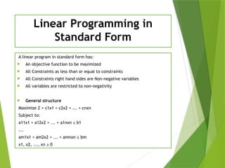
A linear program in standard form has:
 An objective function to be maximized
 All Constraints as less than or equal to constraints
 All Constraints right hand sides are Non-negative variables
 All variables are restricted to non-negativity
 General structure
Maximize Z = c1x1 + c2x2 + ... + cnxn
Subject to:
a11x1 + a12x2 + ... + a1nxn ≤ b1
...
am1x1 + am2x2 + ... + amnxn ≤ bm
x1, x2, ..., xn ≥ 0

3. Algebraic Representation
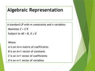
A standard LP with m constraints and n variables:
Maximize Z = C X
ᵀ
Subject to AX = B, X ≥ 0
Where
A is an m×n matrix of coefficients
B is an m×1 vector of constants
C is an n×1 vector of coefficients
X is an n×1 vector of variables

4. Setting up the Simplex
Method
1. Convert inequalities to equalities using slack variables.
2. Form the initial simplex tableau.
3. Identify entering and leaving variables.
4. Perform pivot operations to improve objective function.
5. Iterate until optimal solution is found or unbounded.

5. Structure of the Simplex
Algorithm
1. Start with an initial basic feasible solution.
2. Compute Z-row (objective function row).
3. Identify entering variable (most negative in Z-row).
4. Identify leaving variable (minimum ratio test).
5. Pivot to form next tableau.
6. Repeat until no negative values in Z-row.

6. Definitions of Solutions
 Solution. Any assignment of values to variables
satisfying constraints.
 Corner Point Feasible Solution. A solution at a vertex
of the feasible region.
 Feasible Corner Point Solution. A corner point that
satisfies all constraints.
 Adjacent Corner Point Feasible Solutions. Connected
via a single pivot (exchange of one basic variable).

7. Key Properties of Linear
Programming
 The optimum point lies at a feasible corner point.
 If a corner point feasible solution has an objective value
better than all adjacent solutions, it is optimal.
 There are a finite number of corner point feasible
solutions.

8. The Simplex Tableau
Definition: a tabular method used in the Simplex
algorithm, a popular procedure for solving linear
programming problems, particularly optimization problems
where the goal is to maximize or minimize a linear
objective function subject to a set of linear inequalities or
equations (constraints).

9. Simplex Tableau Steps
1. Construct initial tableau (objective function and
constraints).
2. Select pivot column (most negative indicator).
3. Select pivot row (minimum positive ratio).
4. Perform row operations to make pivot = 1 and others in
column = 0.
5. Repeat until optimality condition is met.

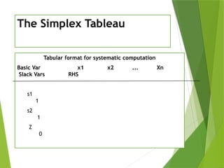
10. The Simplex Tableau
Tabular format for systematic computation
Basic Var x1 x2 ... Xn
Slack Vars RHS
s1
1
s2
1
Z
0

11. Conclusion
 Simplex method provides a systematic approach to
solving LP problems.
 Relies on moving from one corner point to another to
find the optimum.
 Finite, structured, and guarantees an optimal solution if
one exists.
 Efficient and widely used in real-world applications