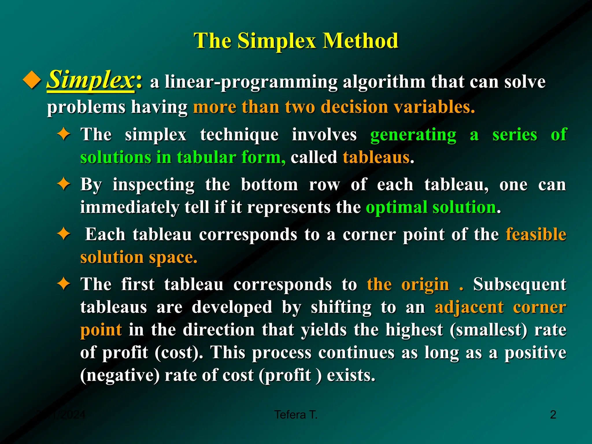
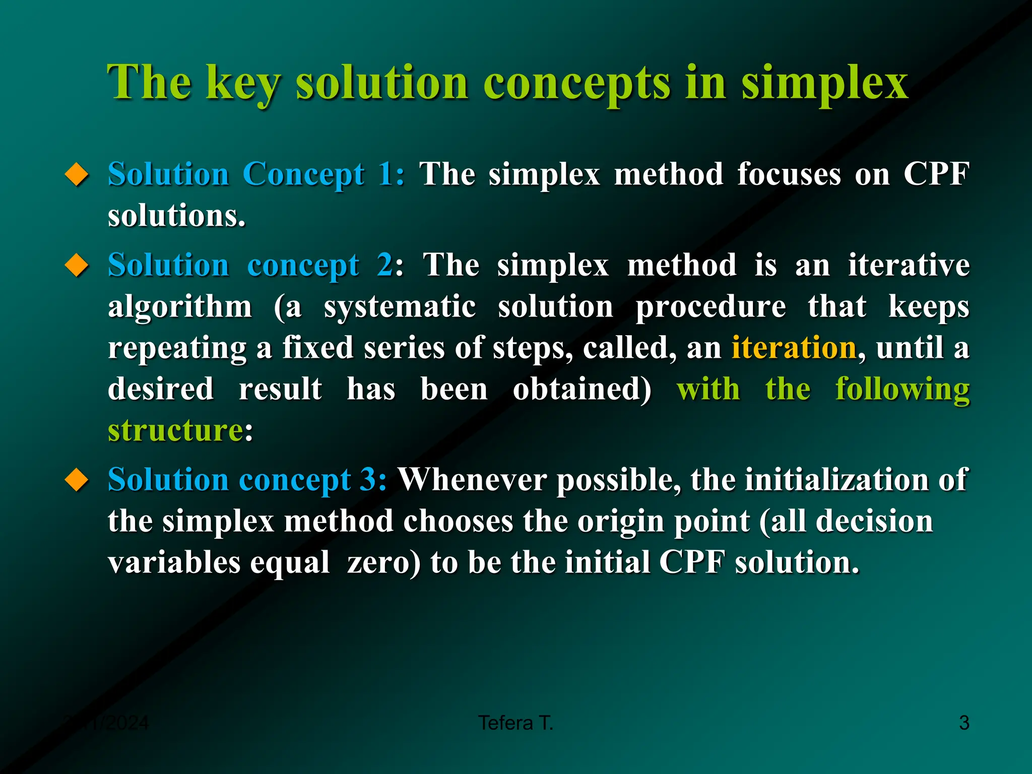
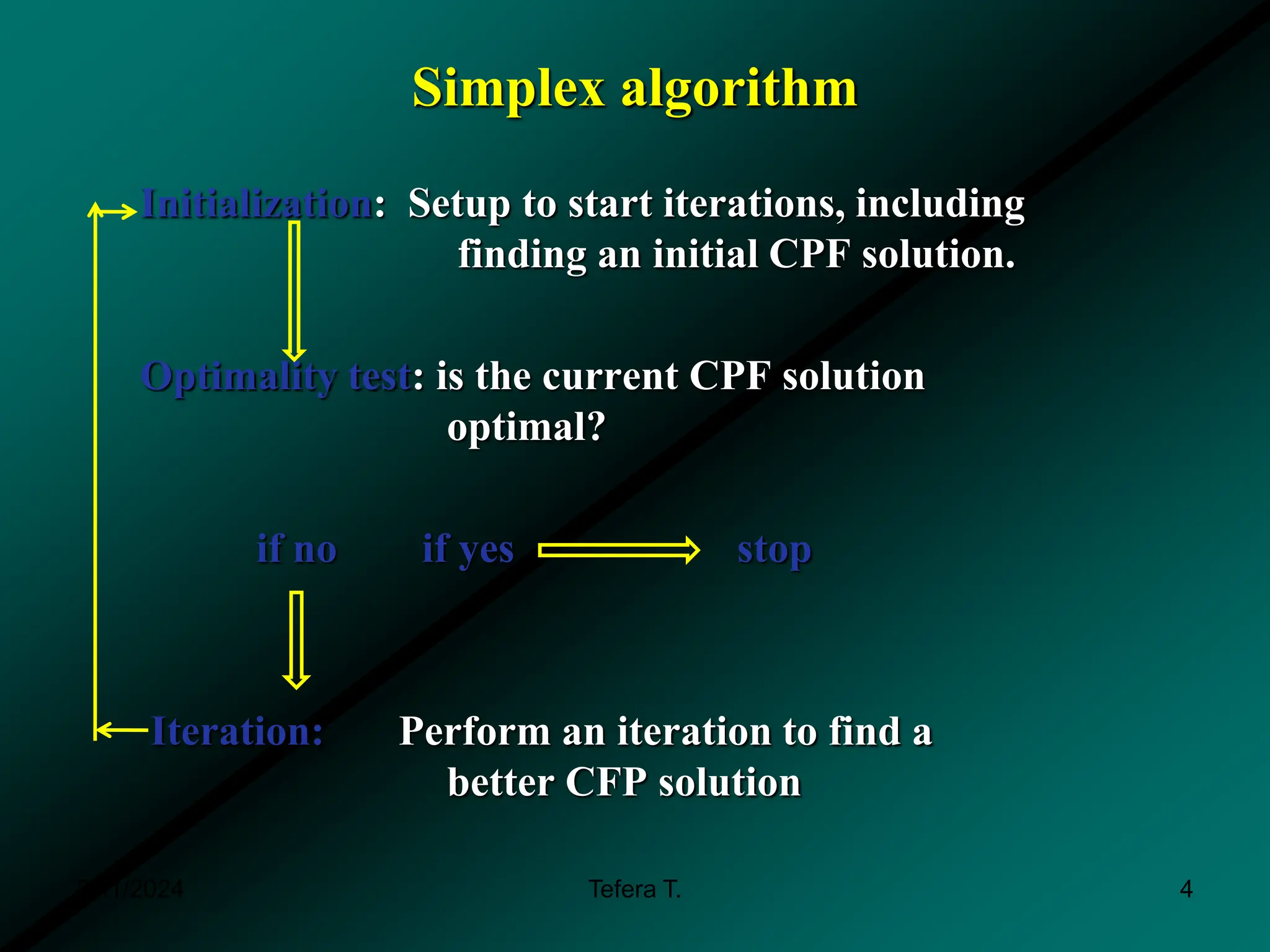
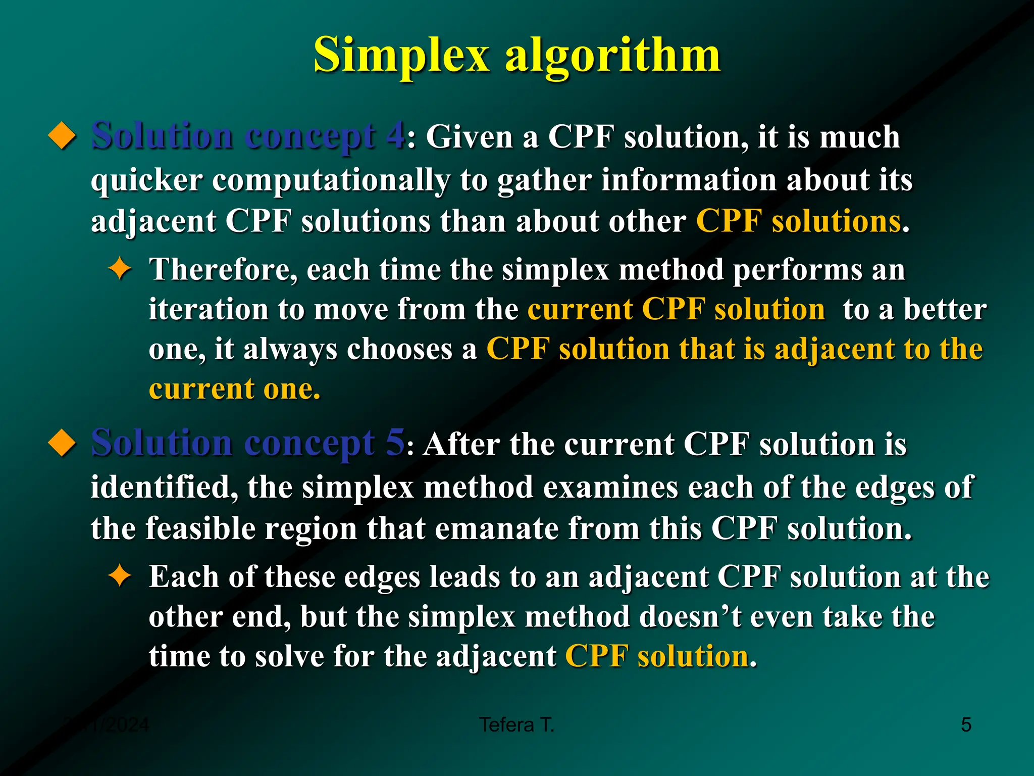
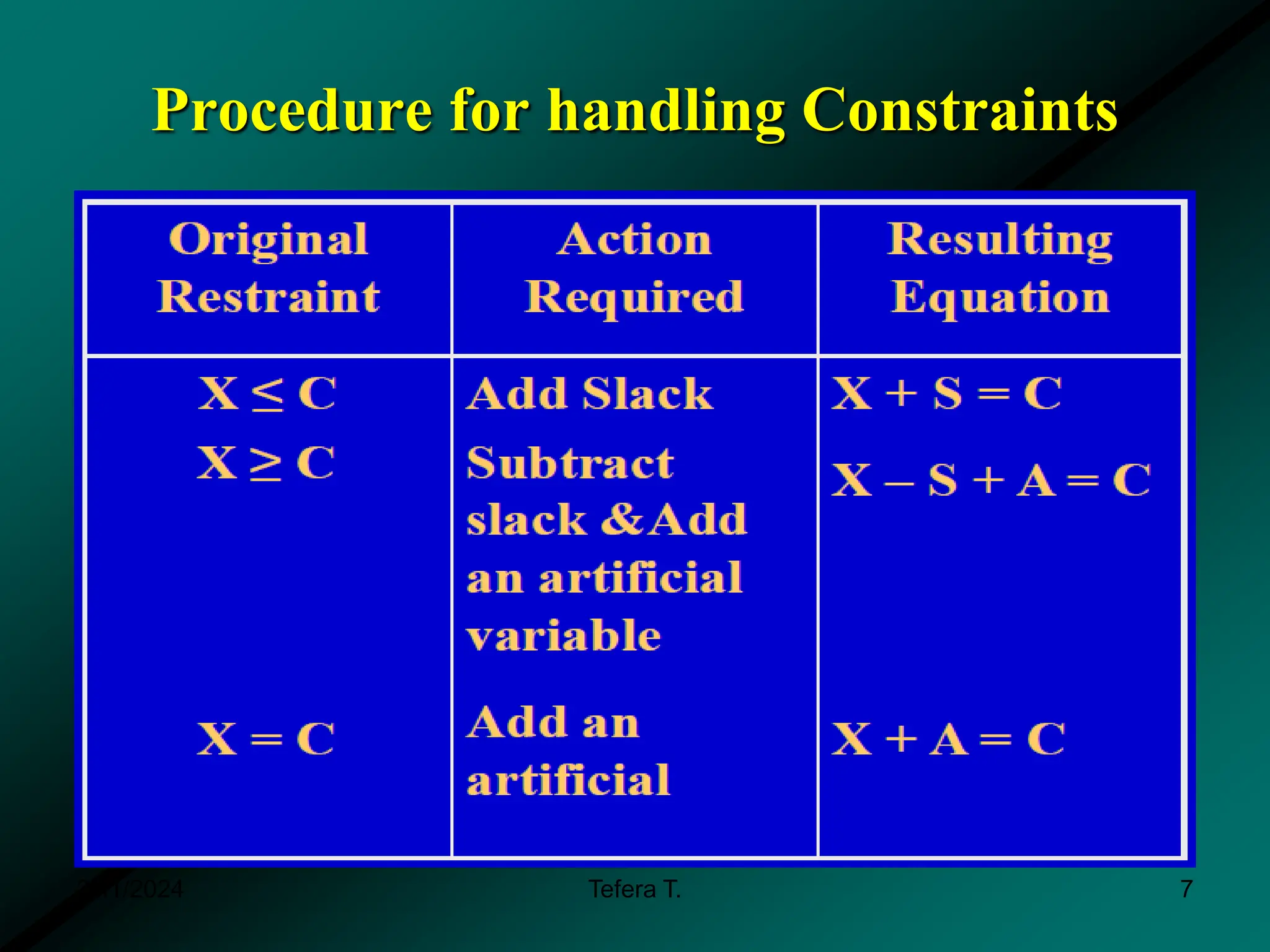
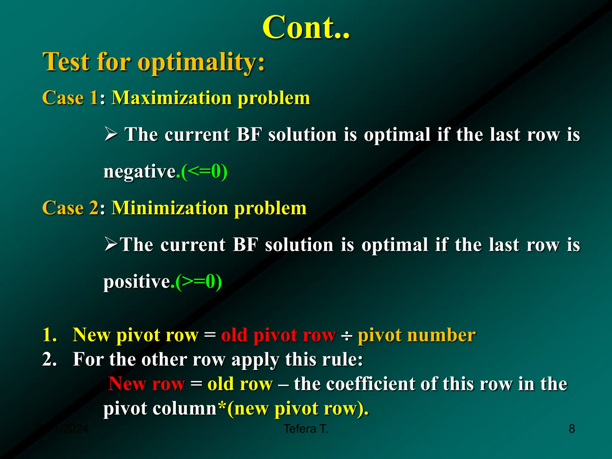
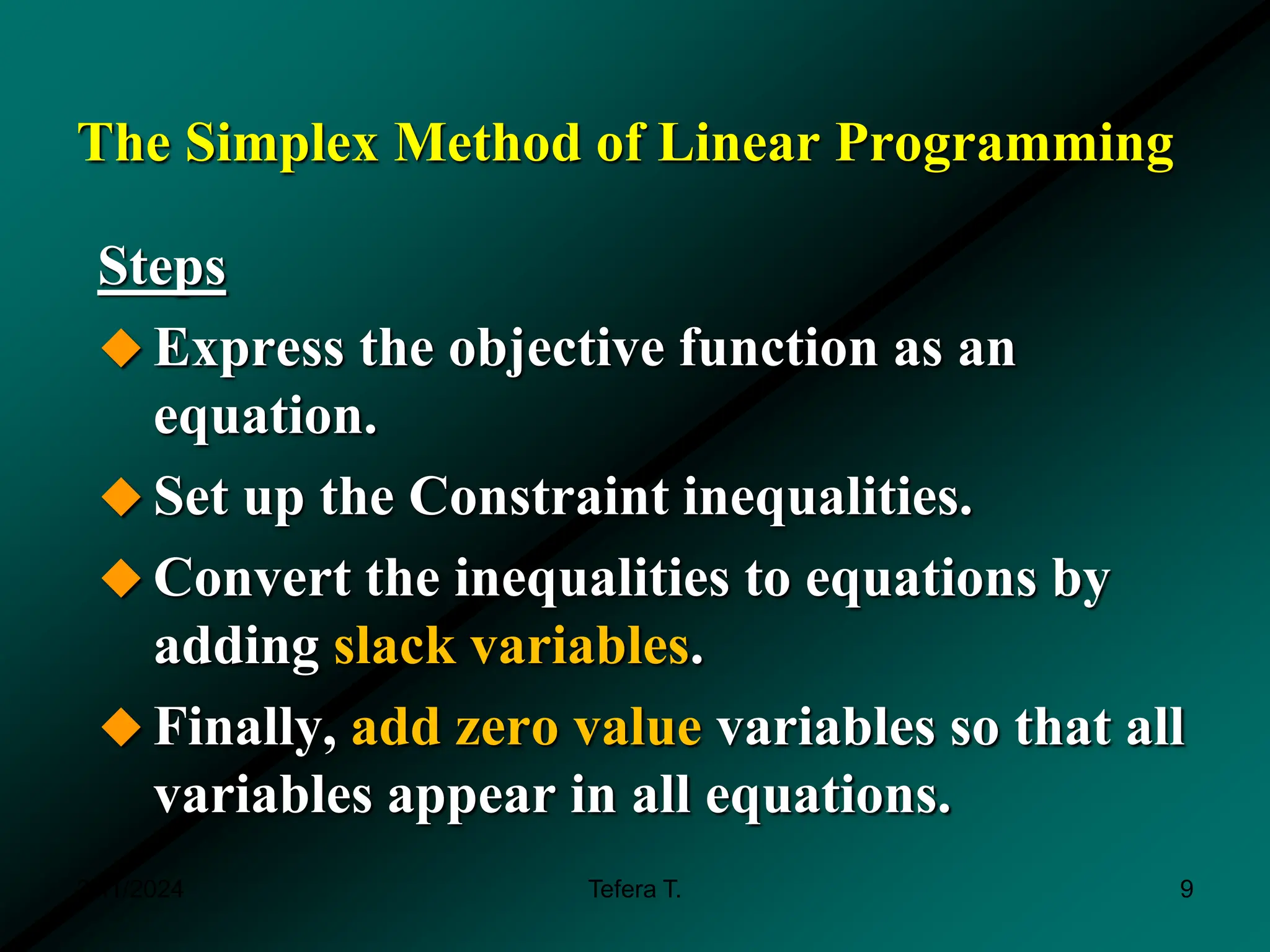
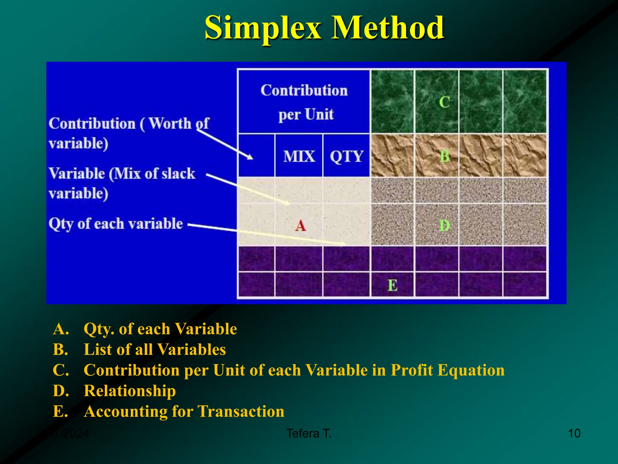
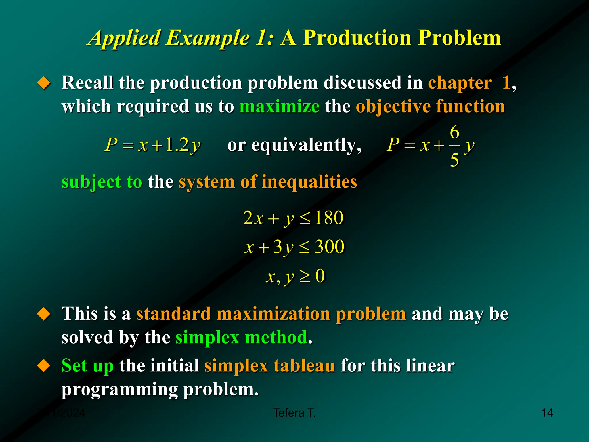
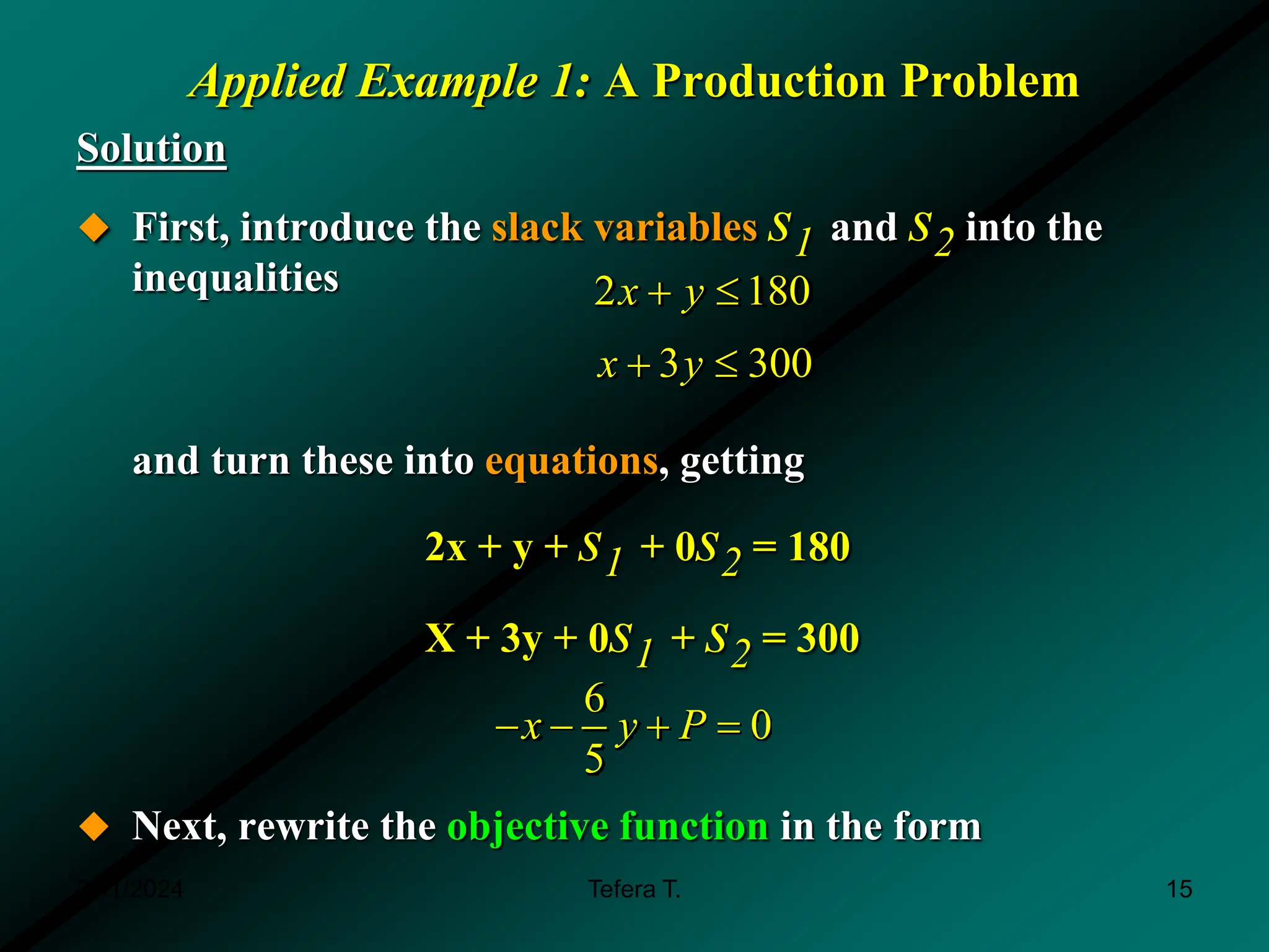
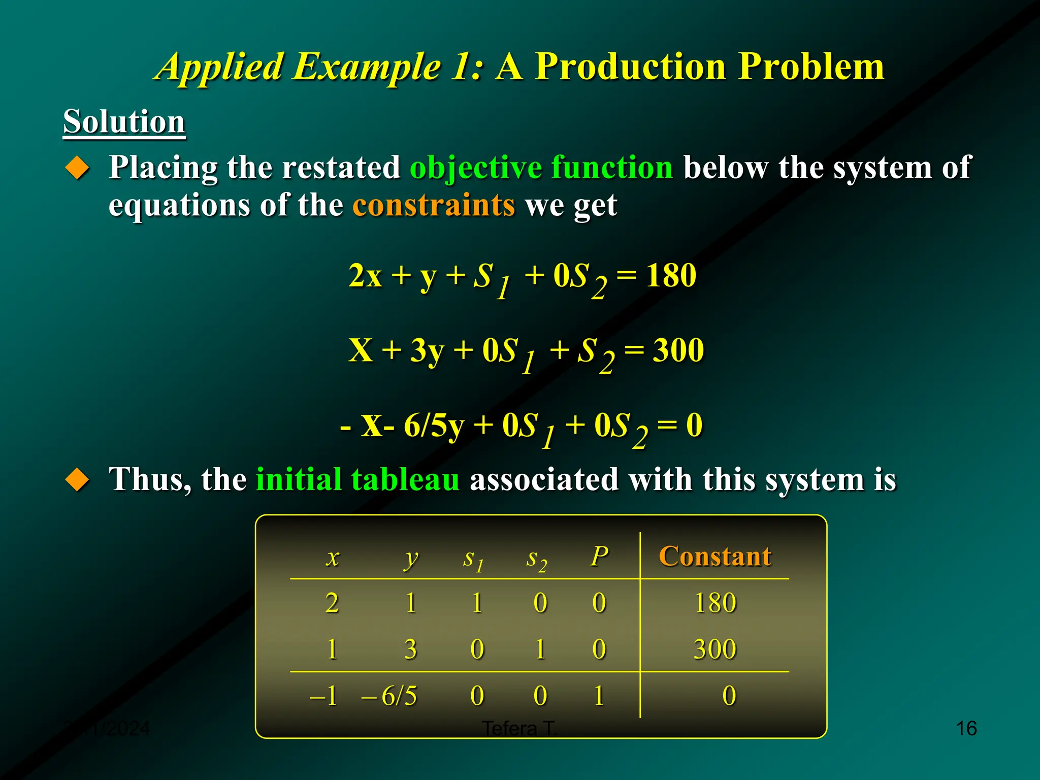
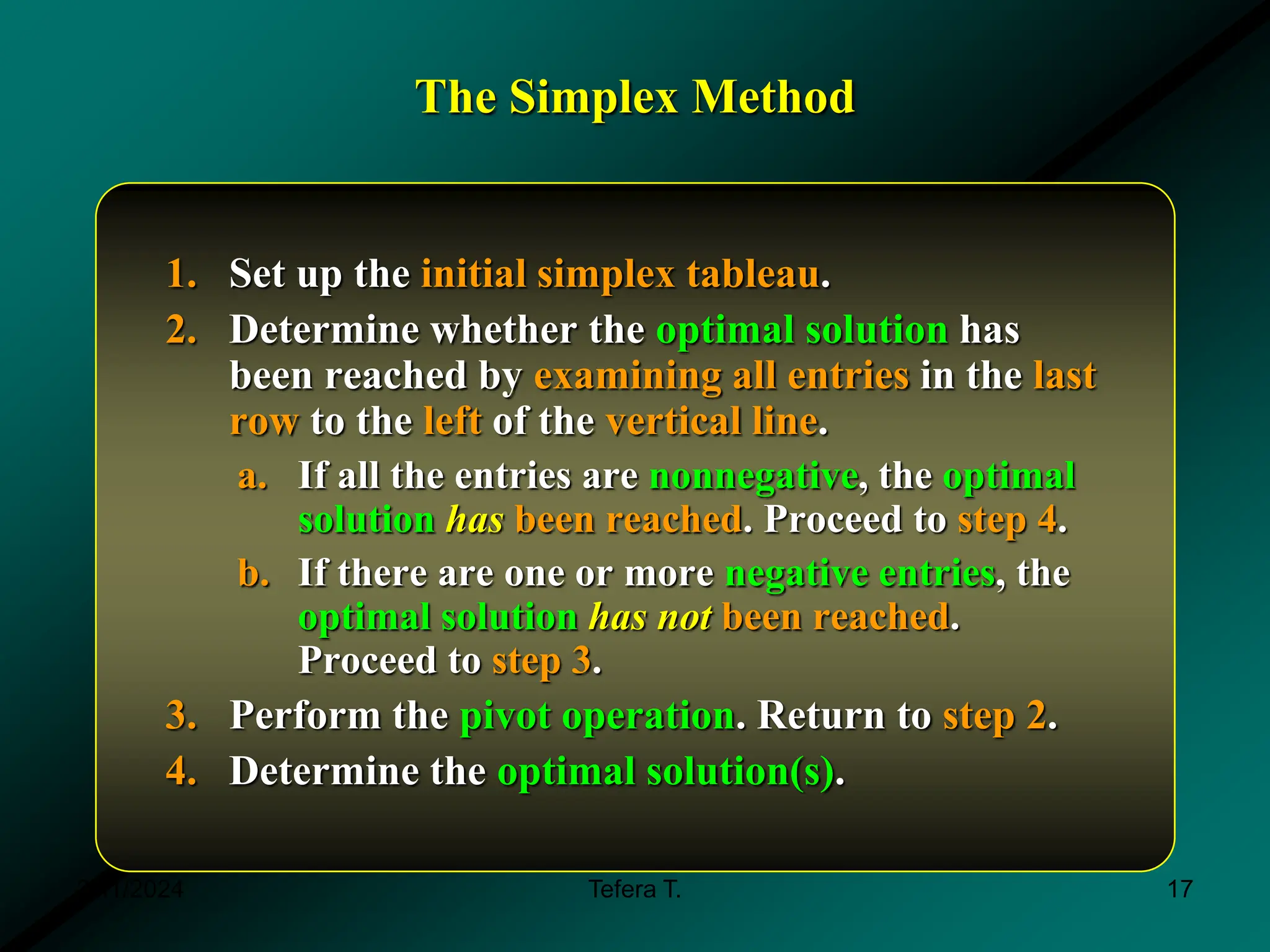
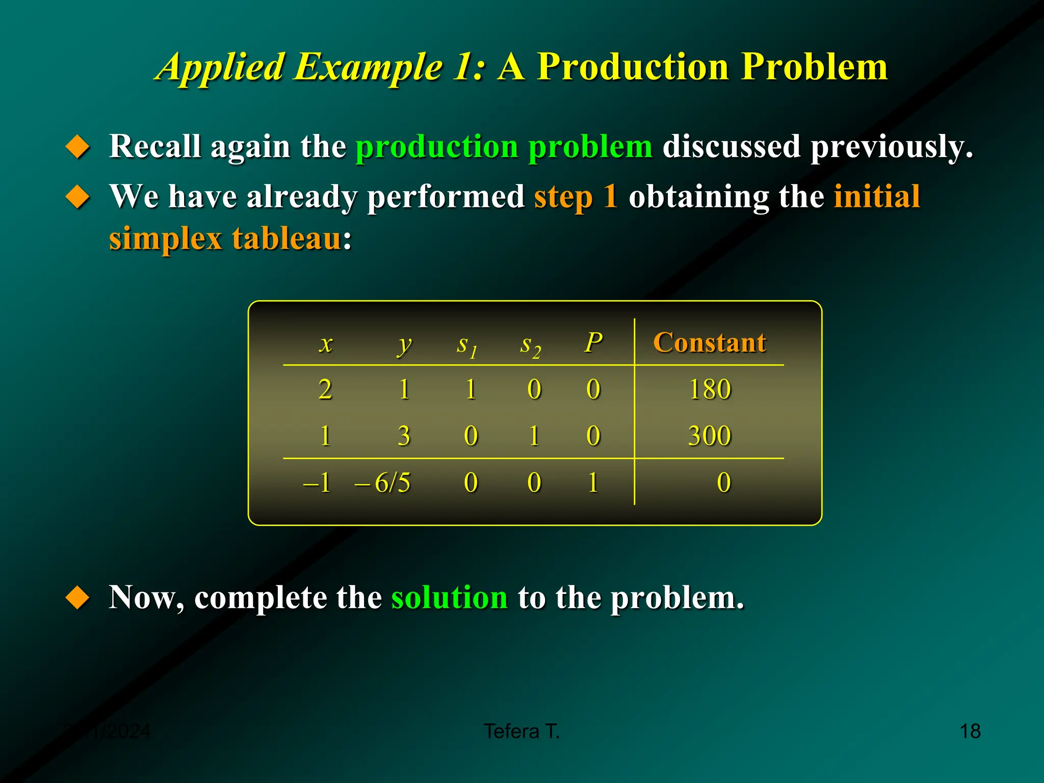
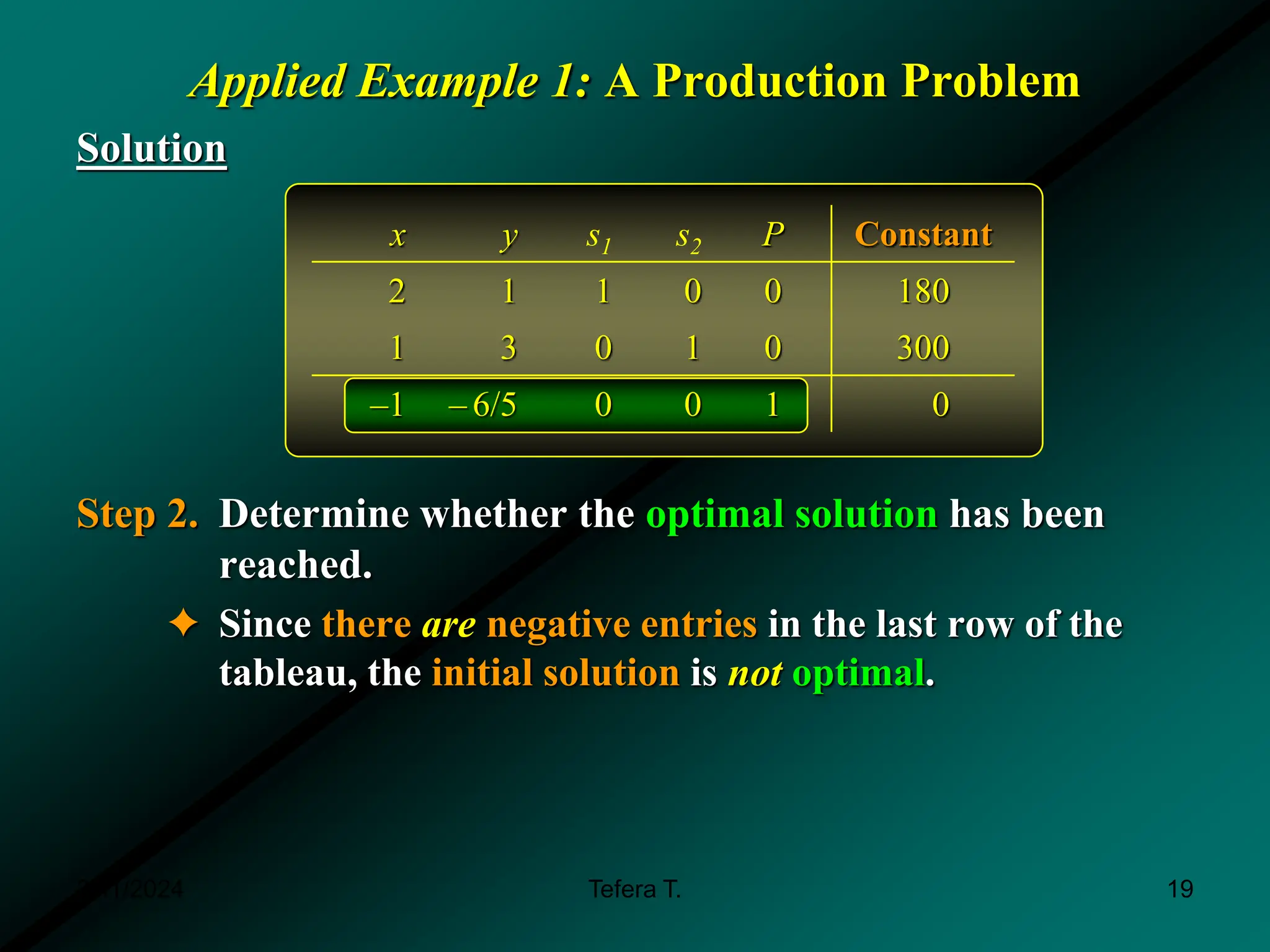
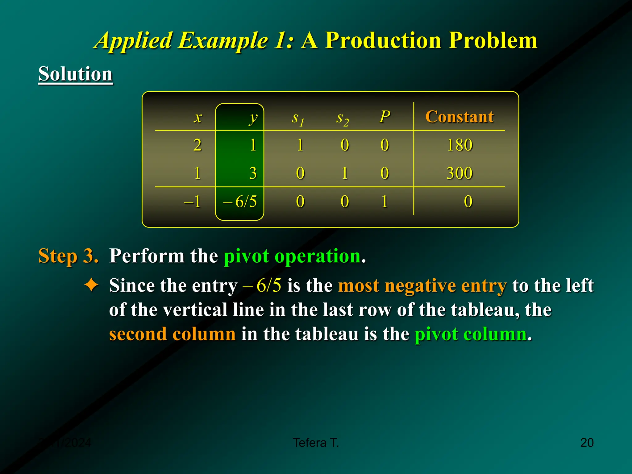
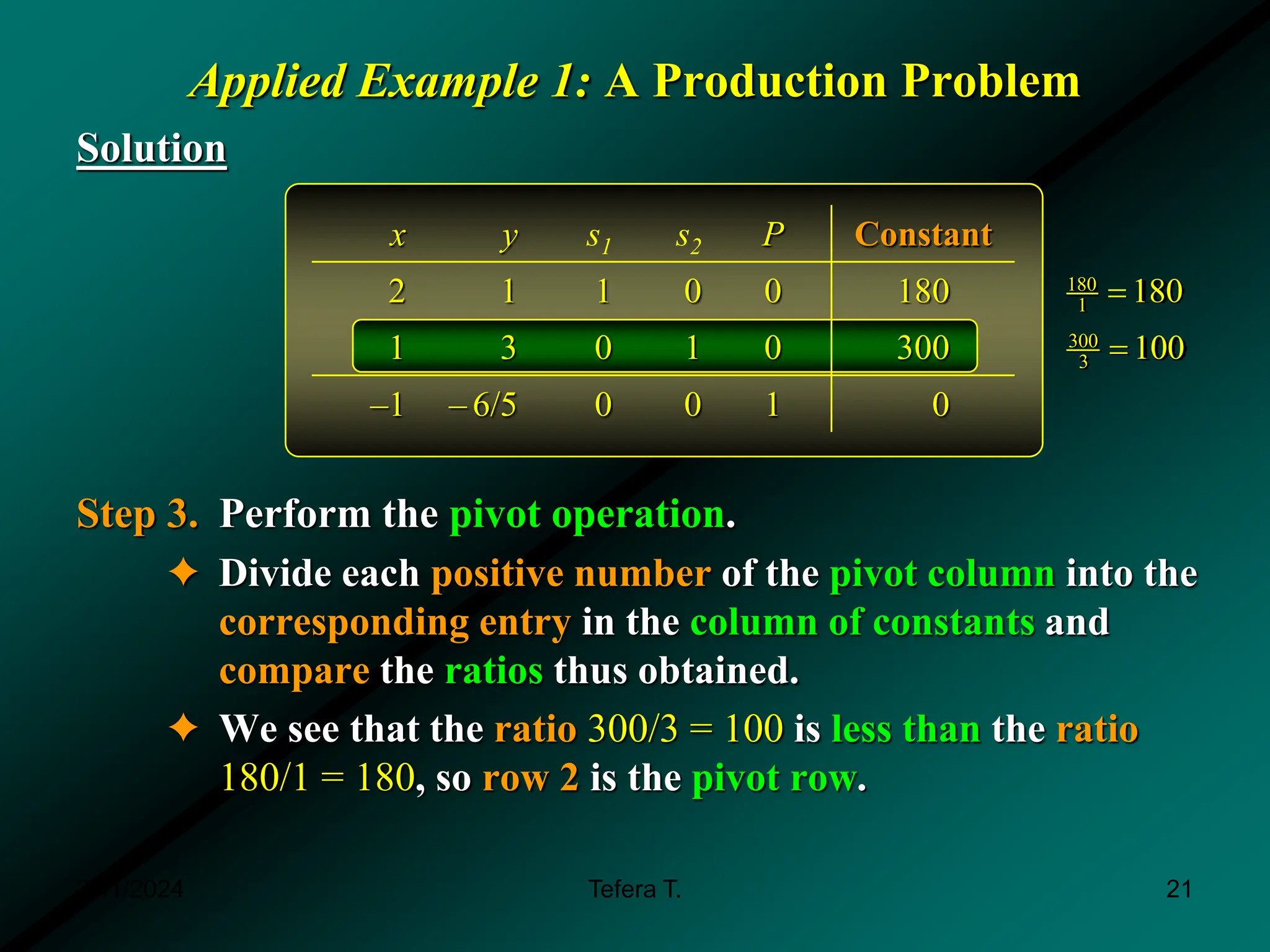
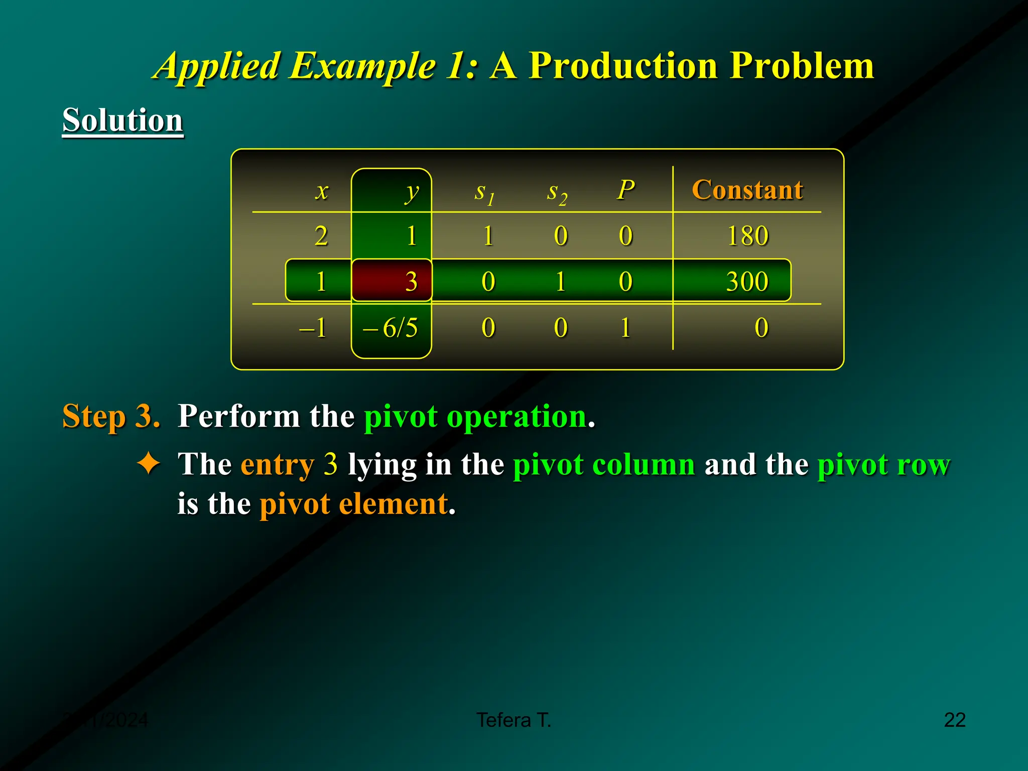
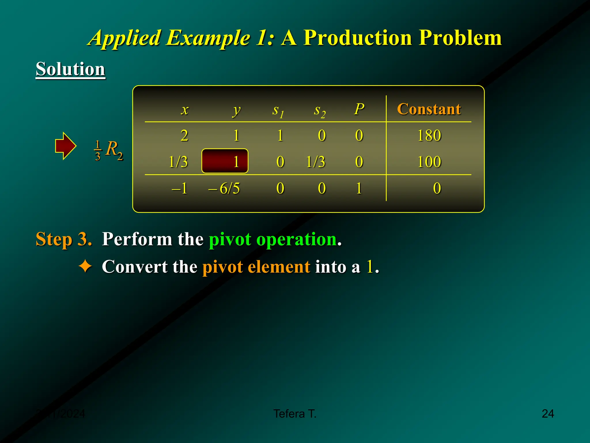
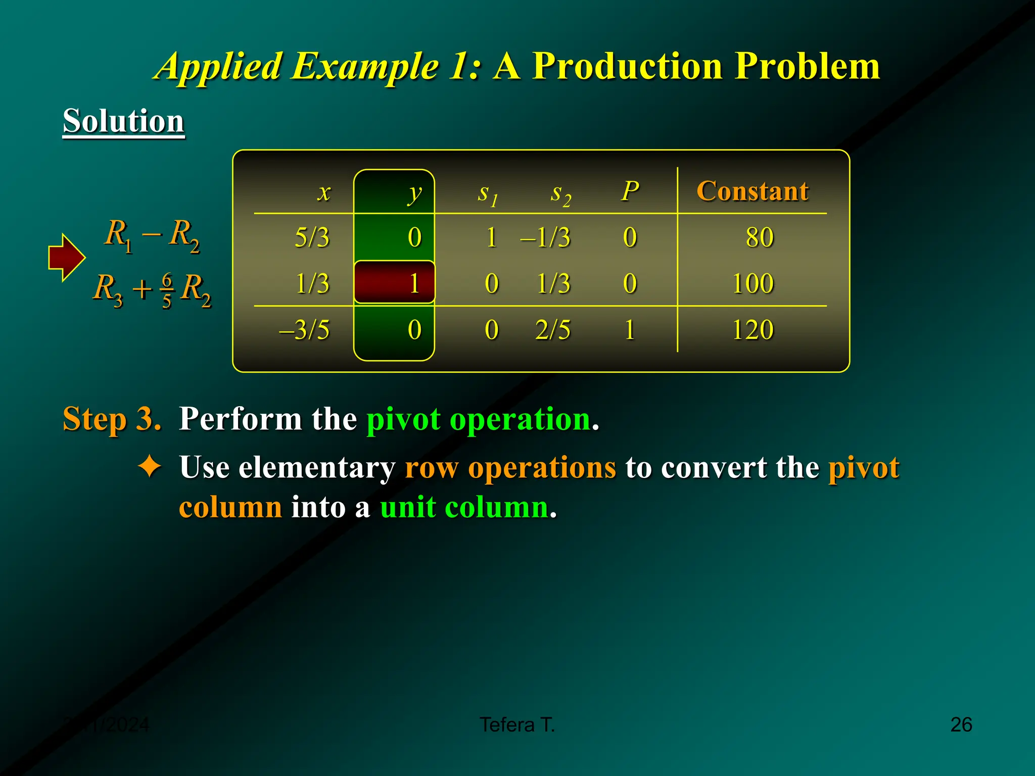
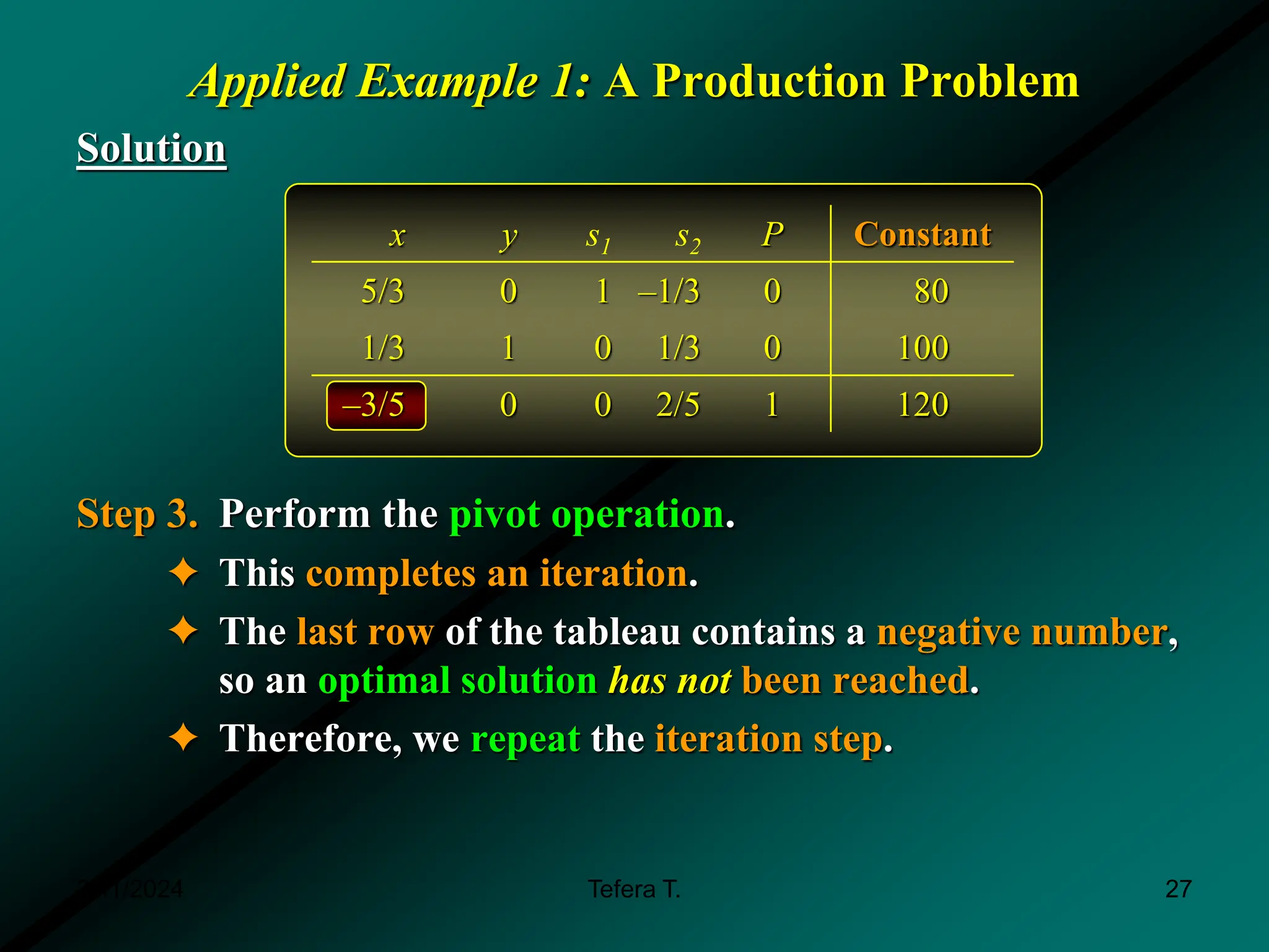
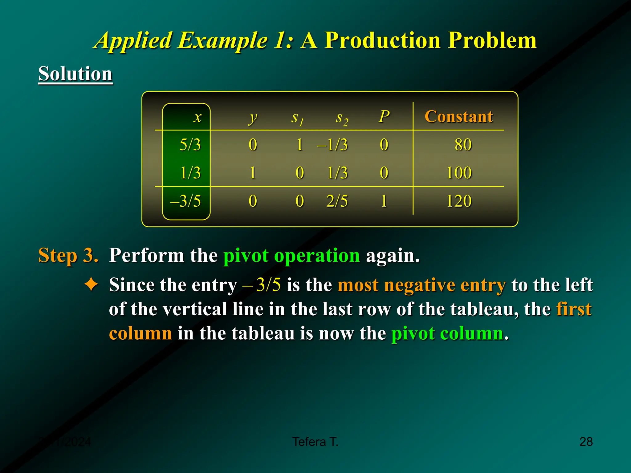
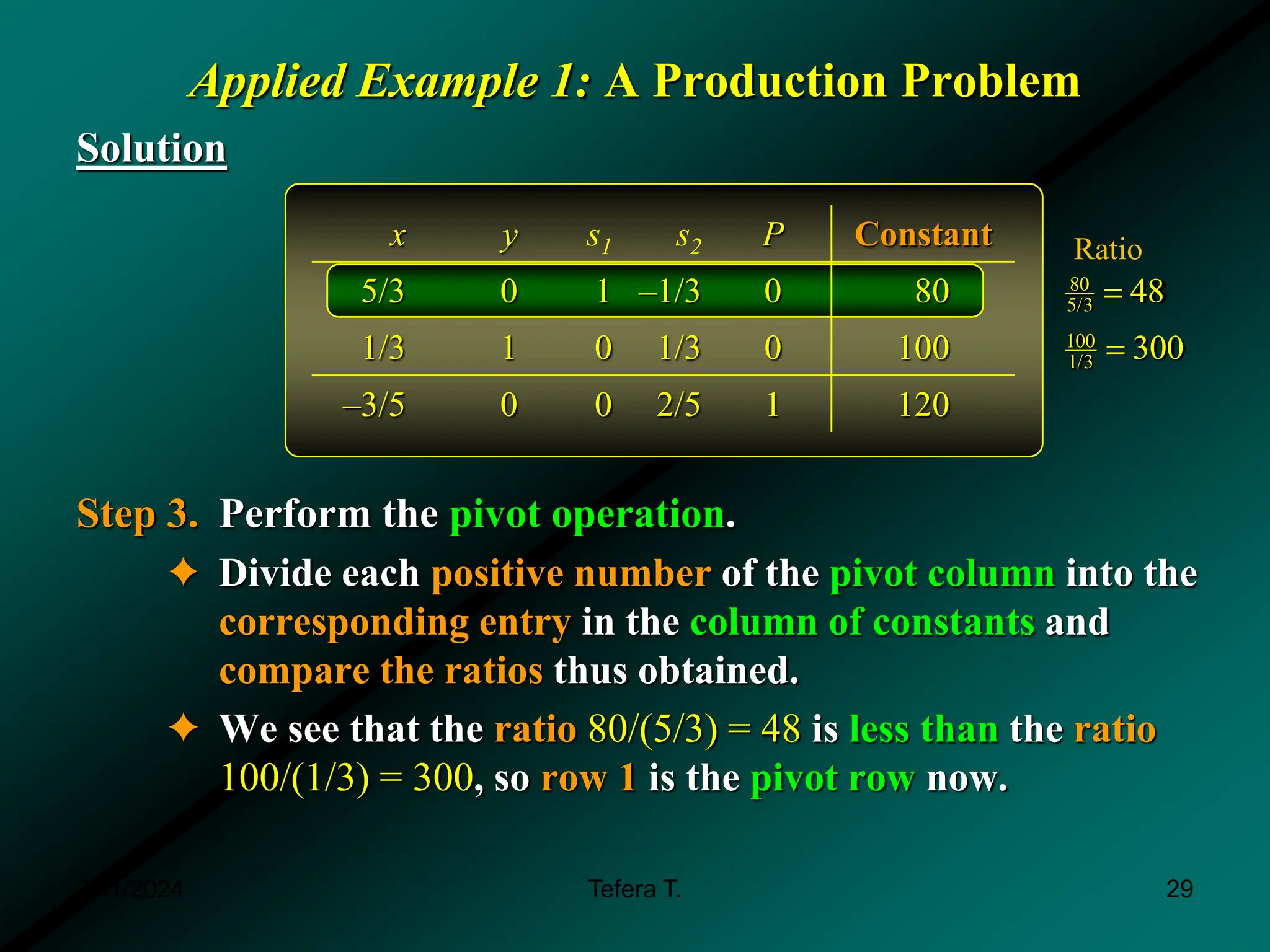
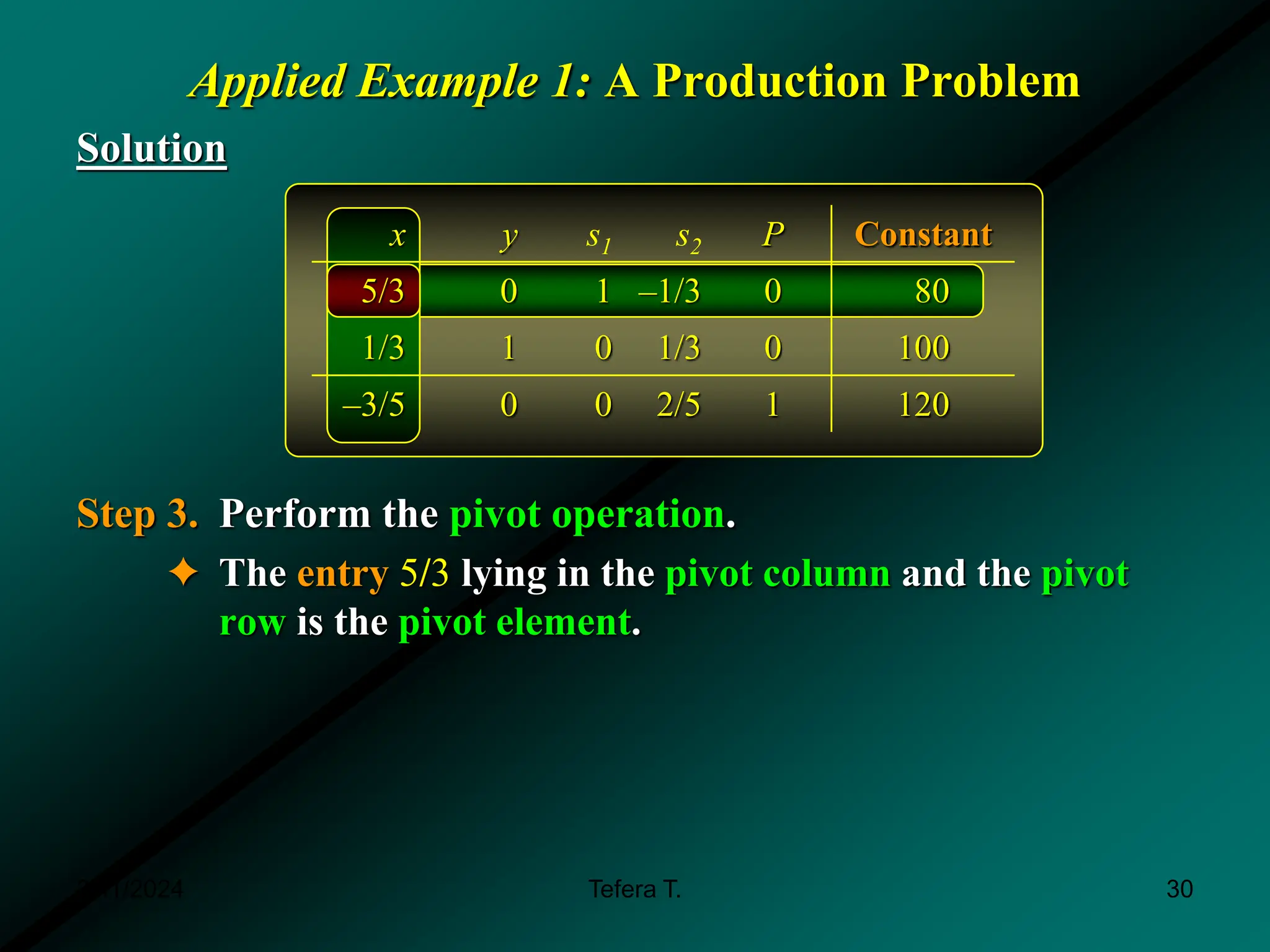
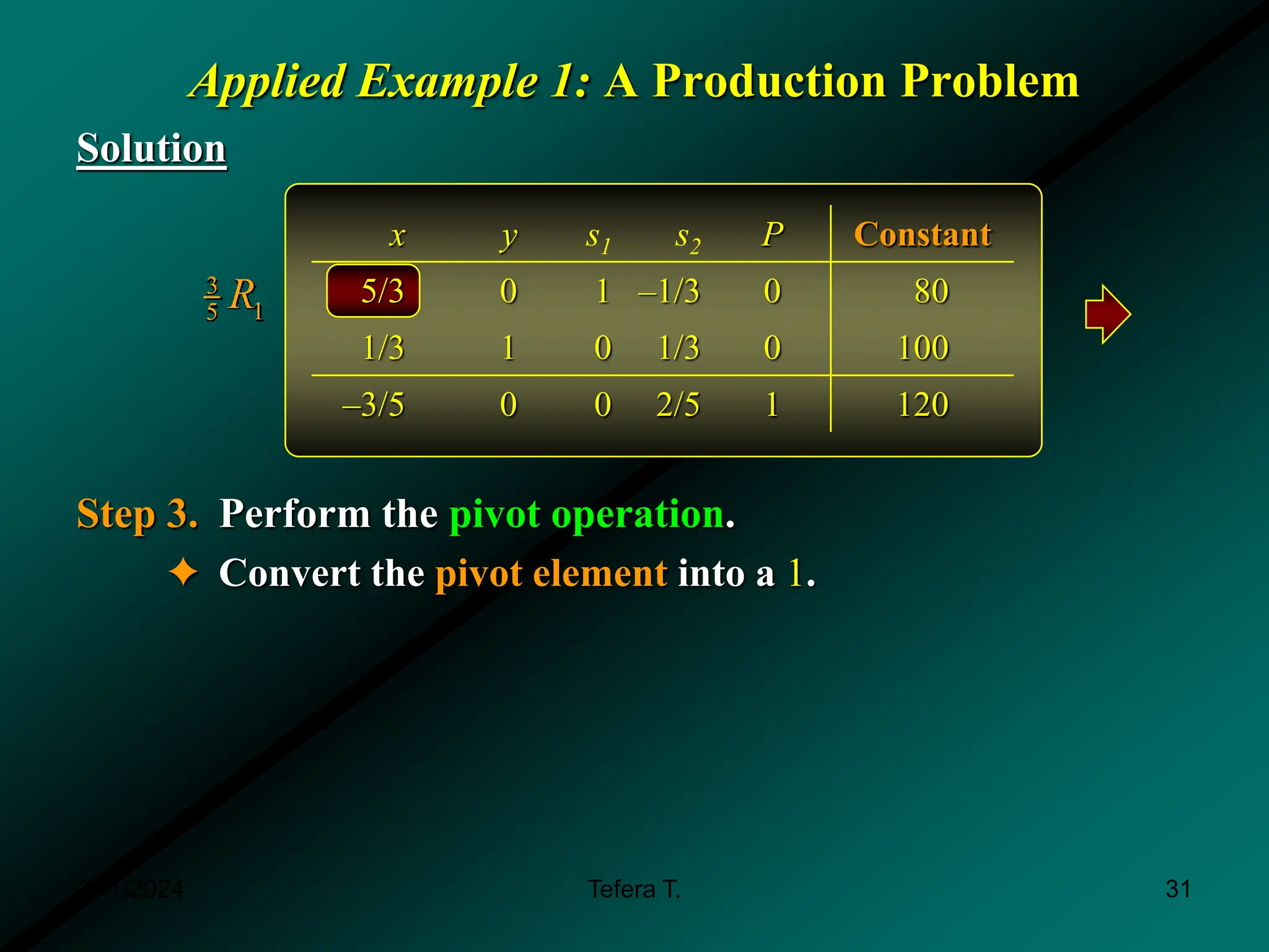
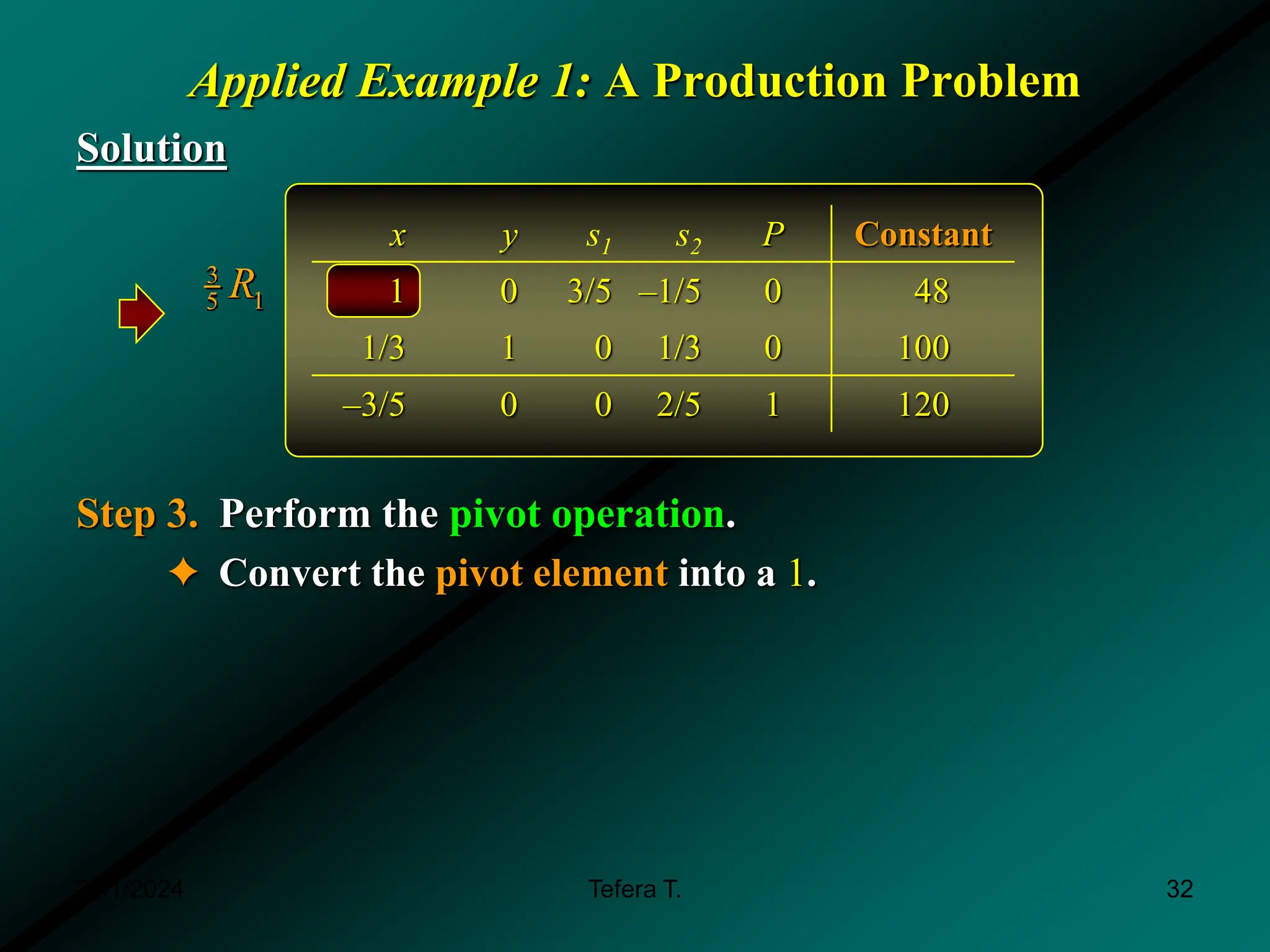
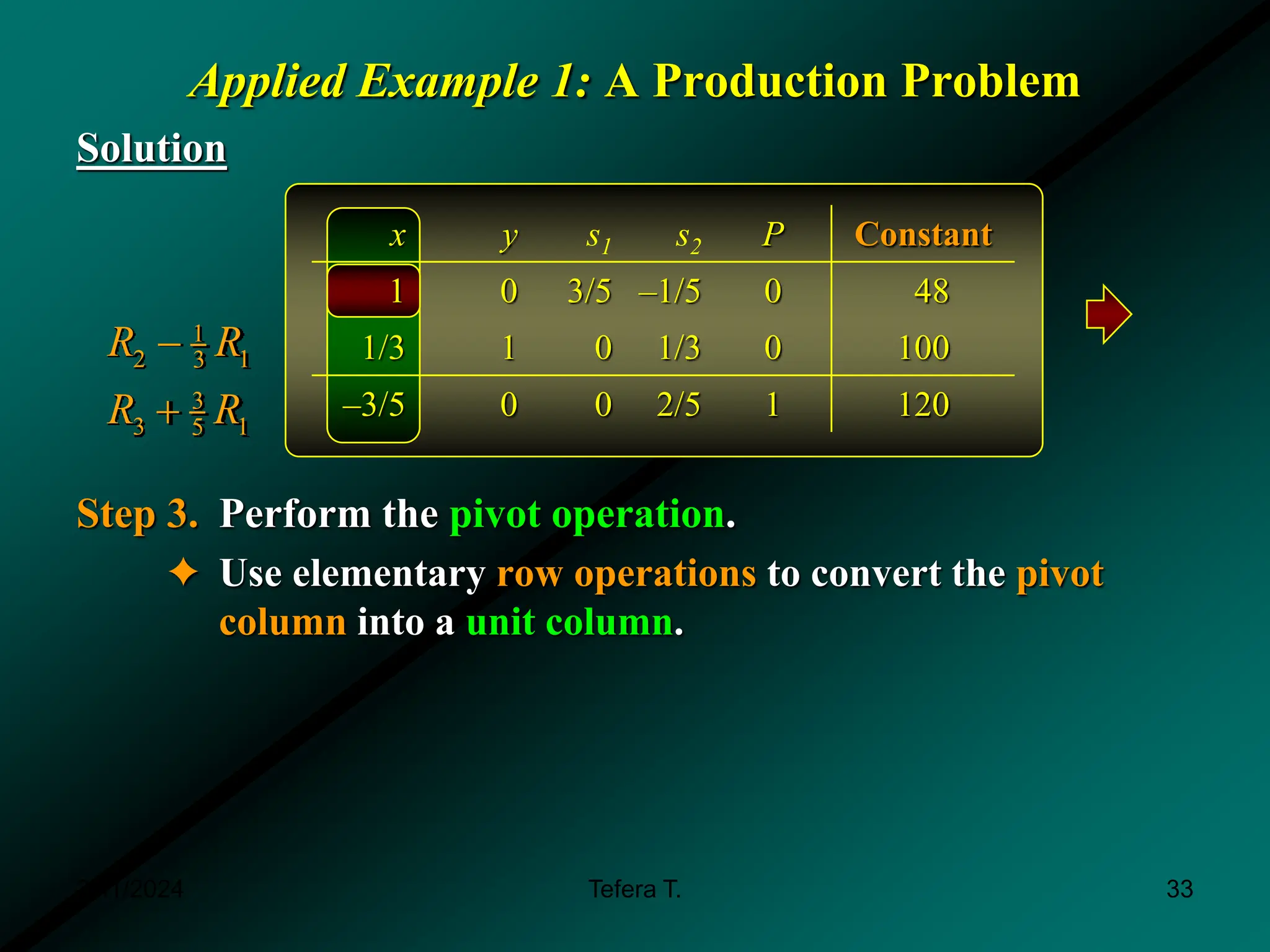
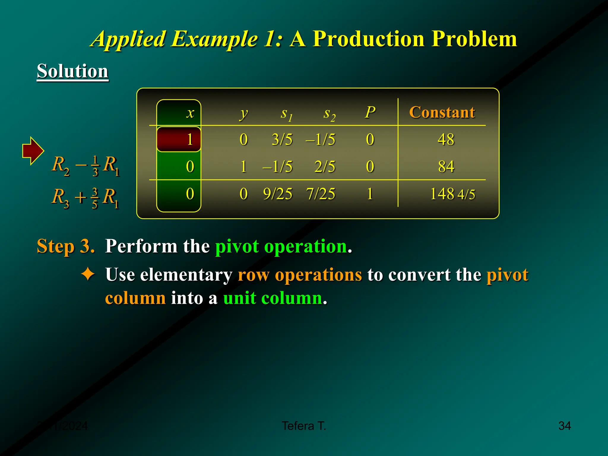
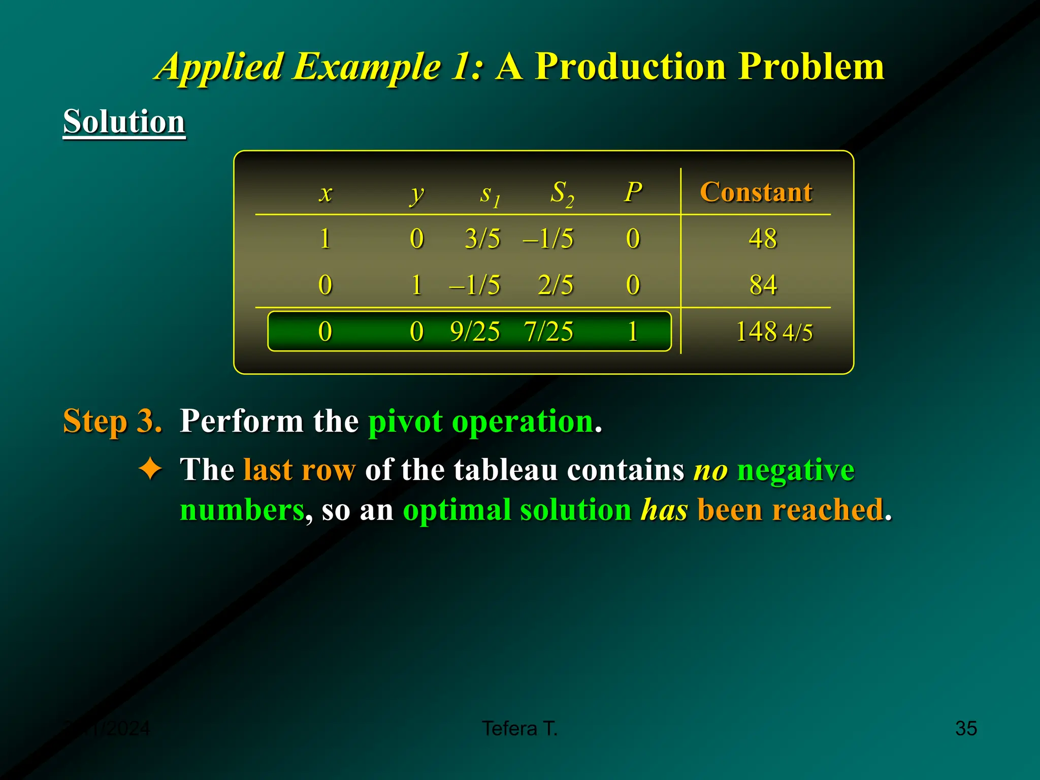
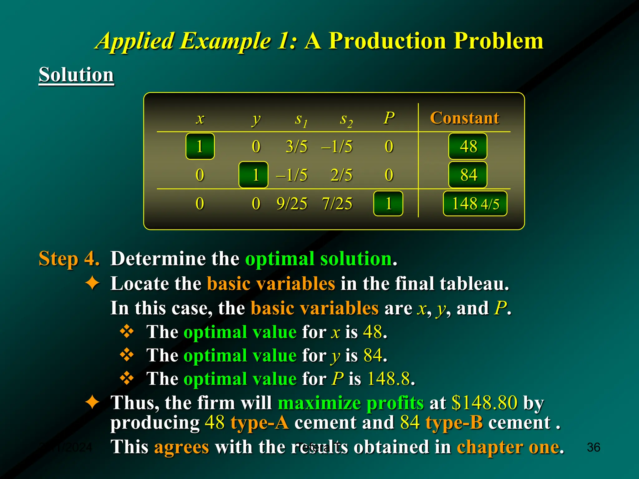
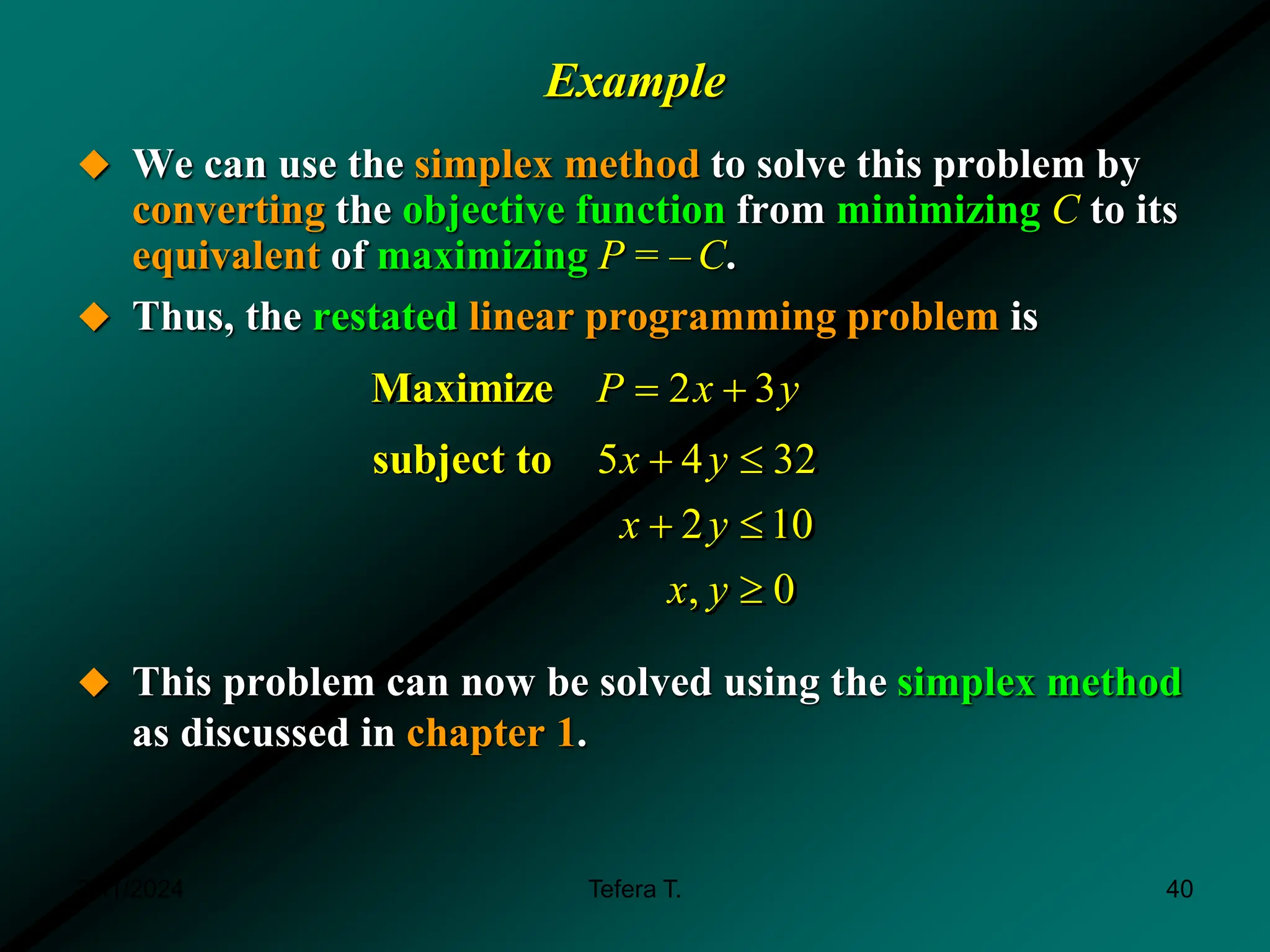
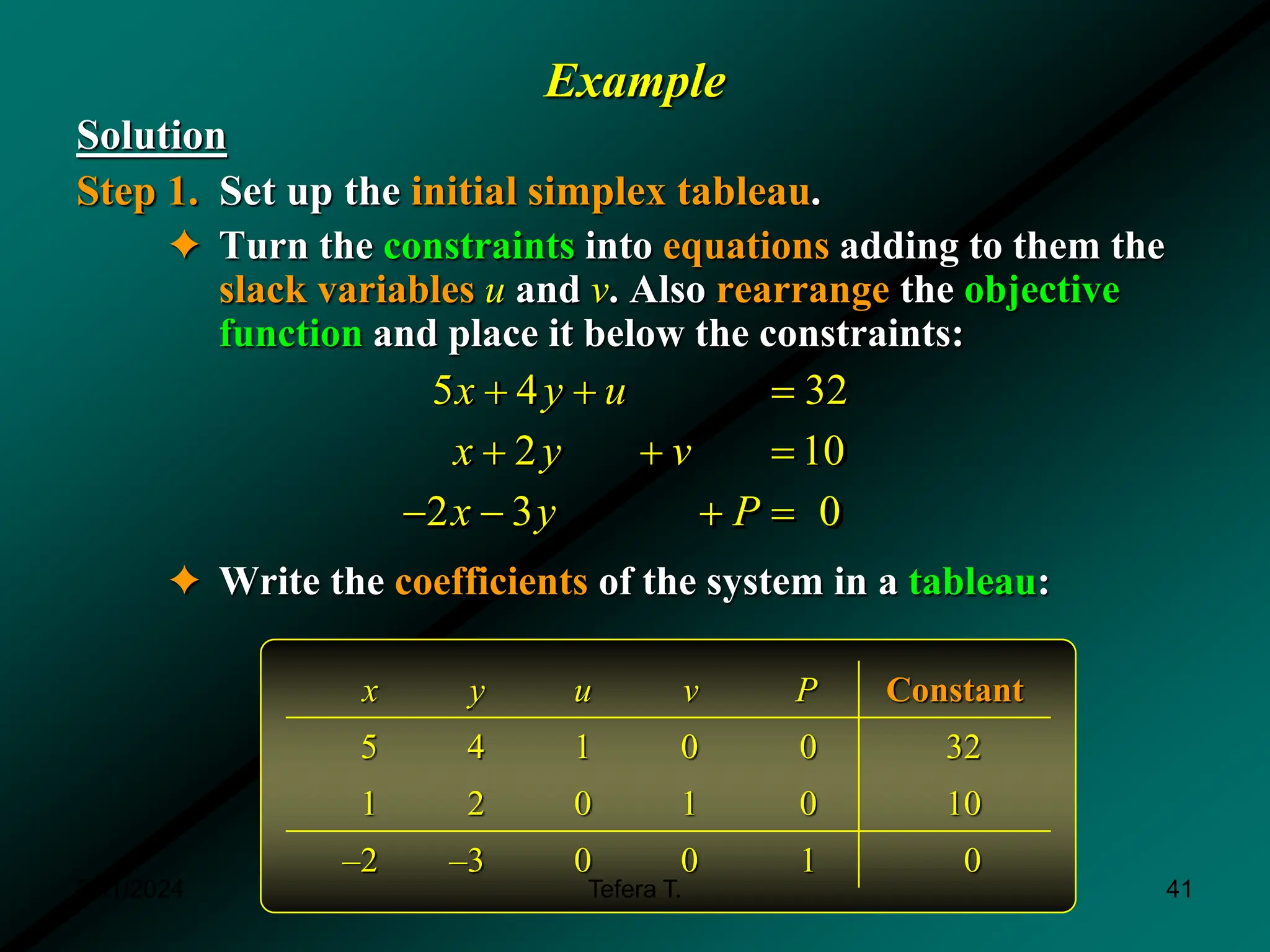
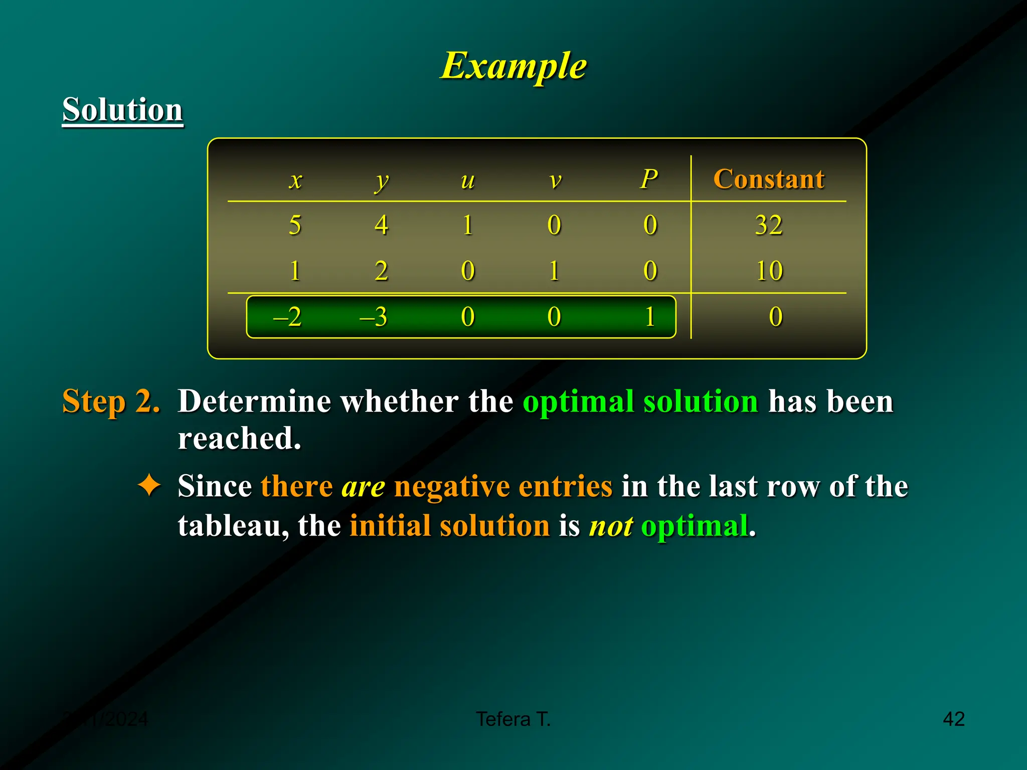
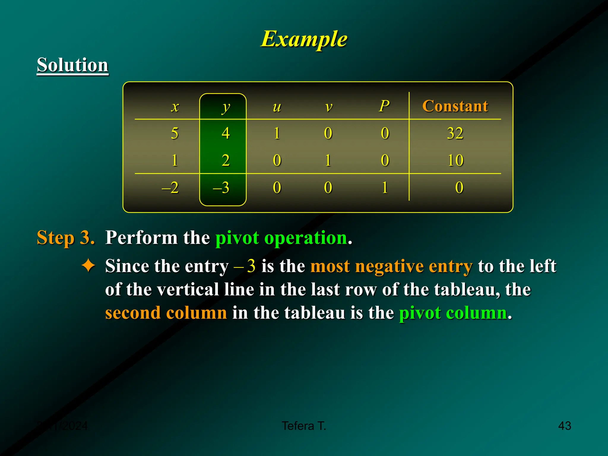
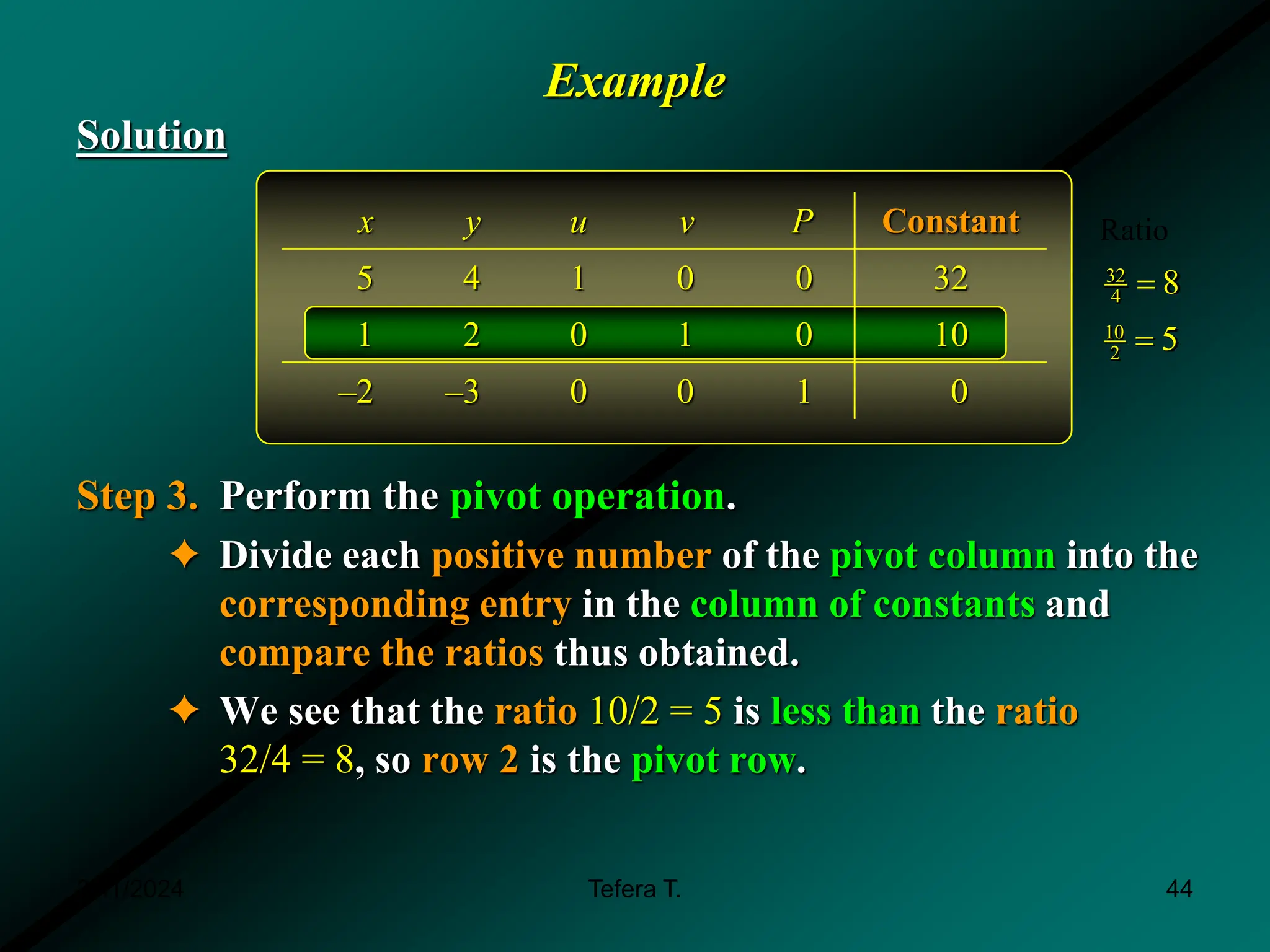
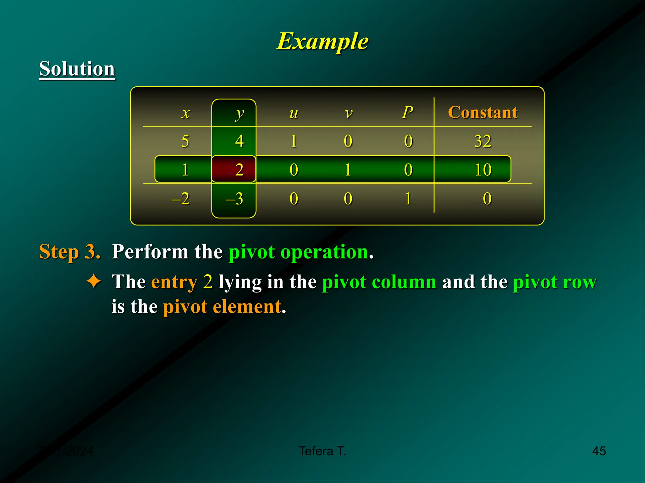
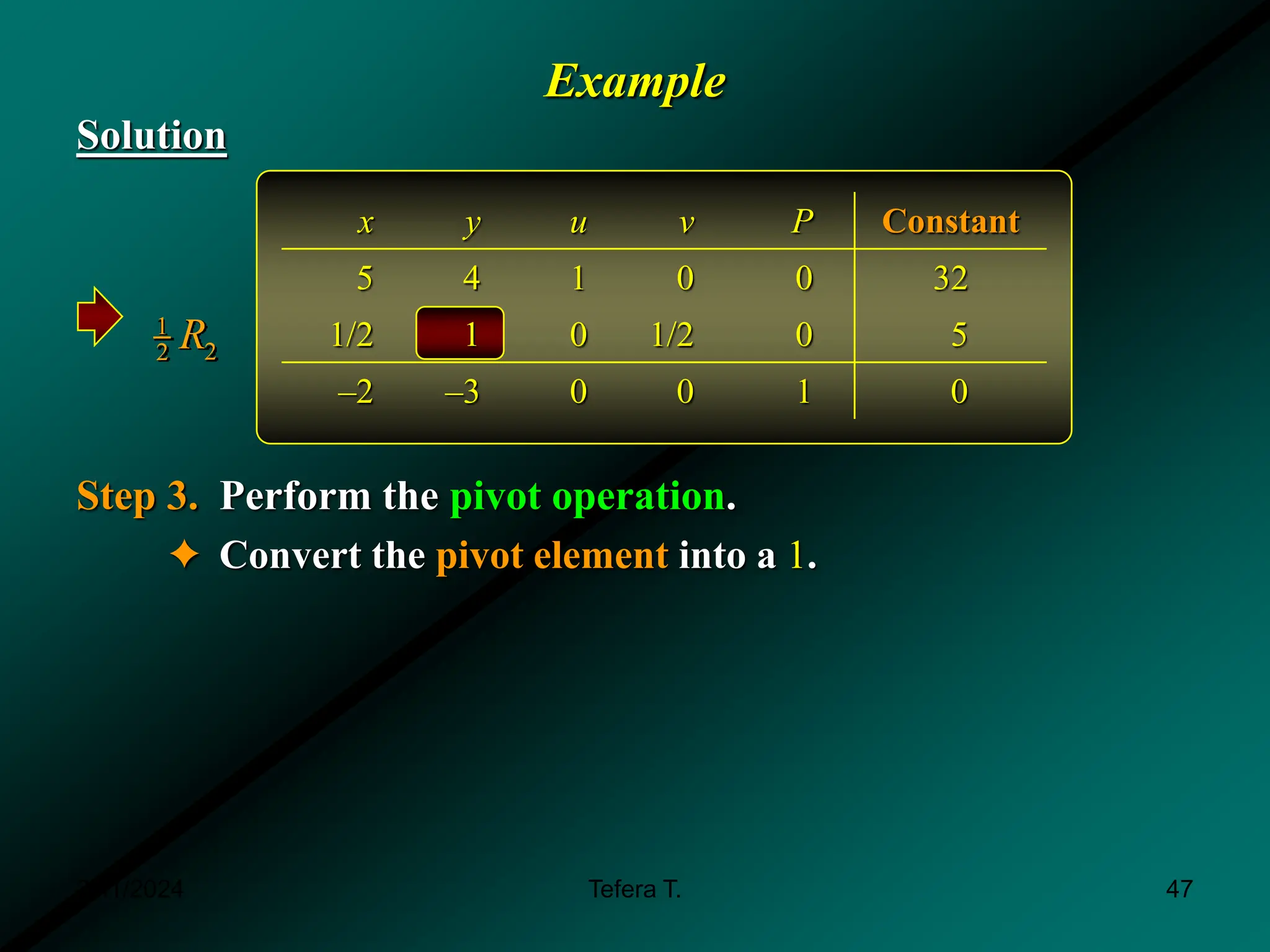
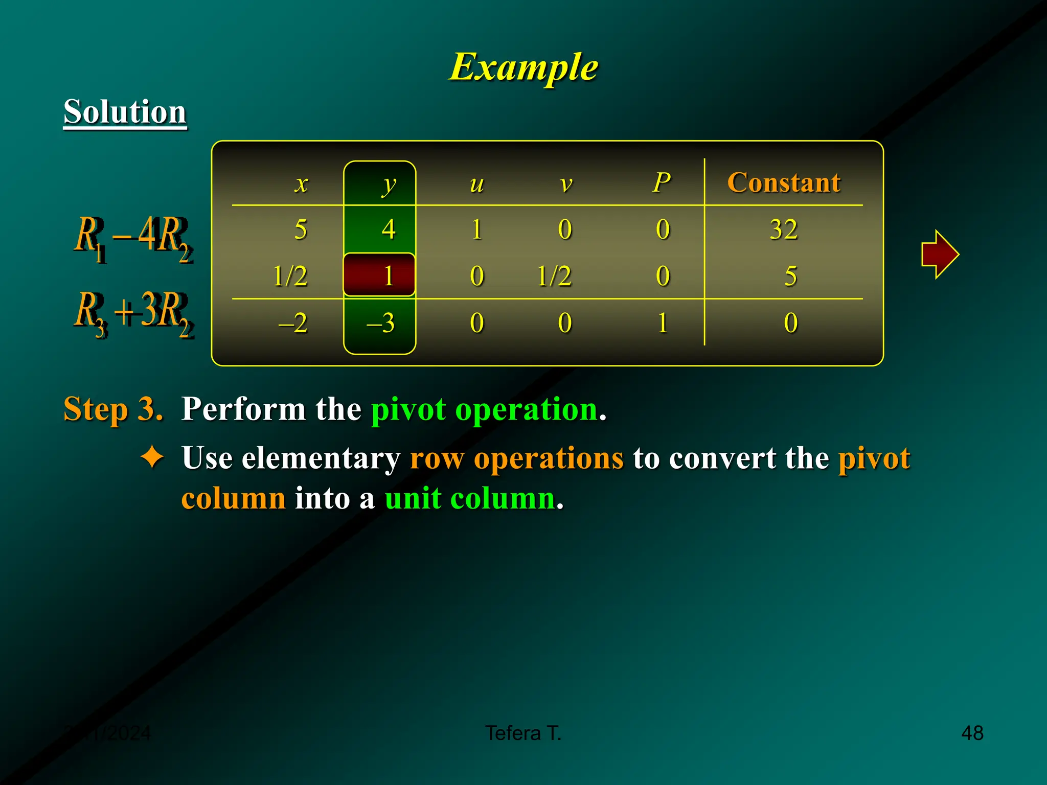
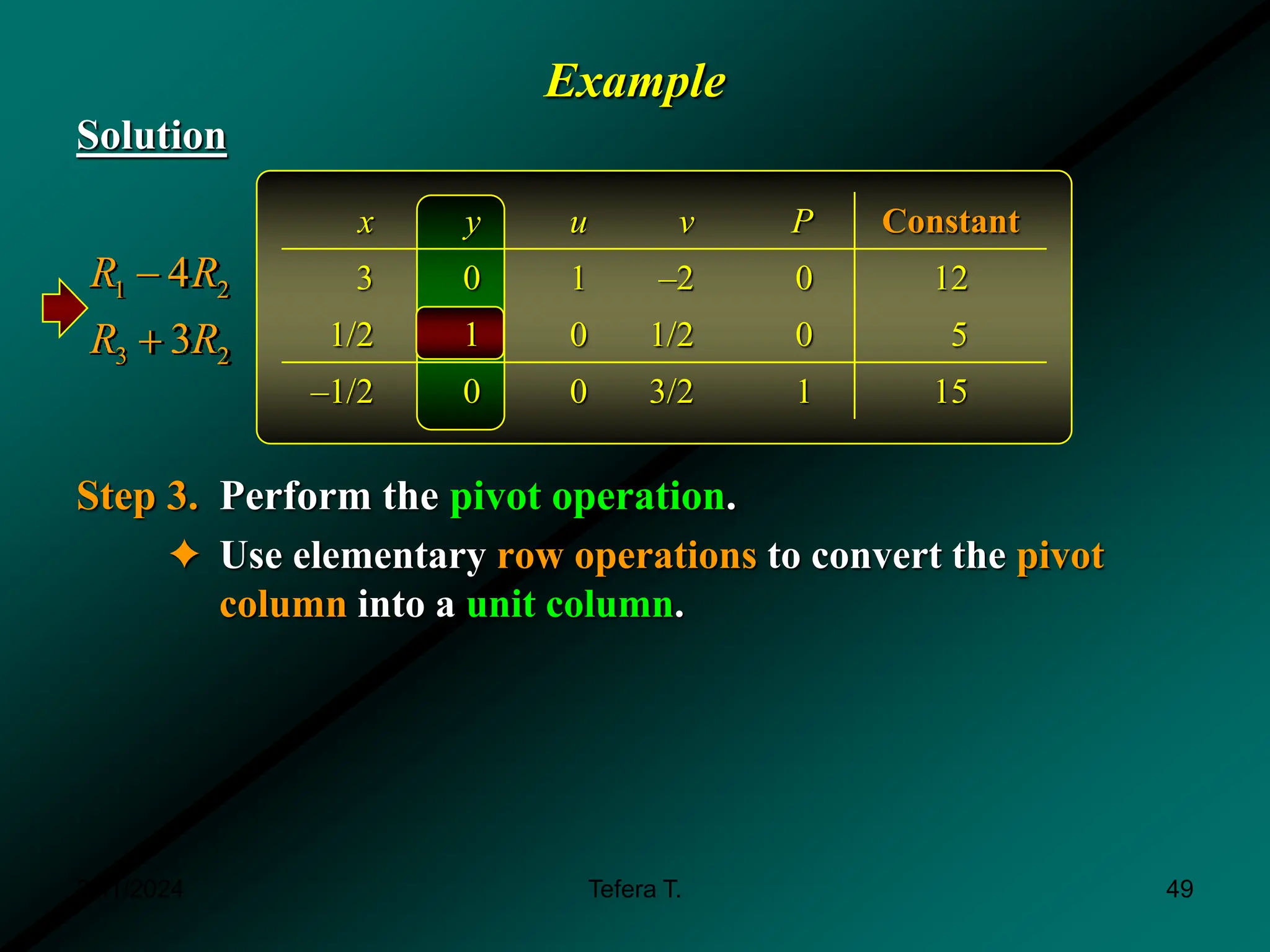
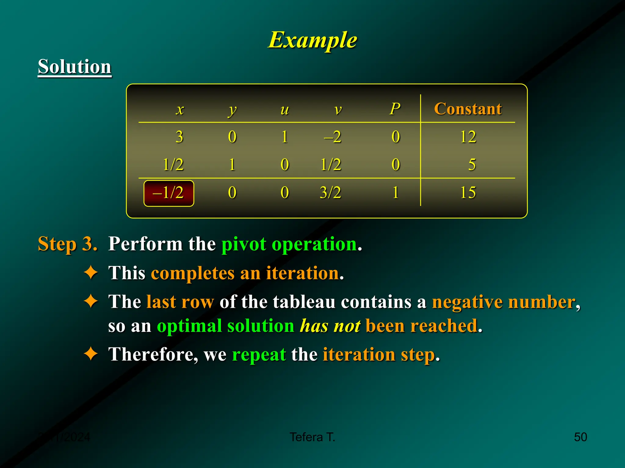
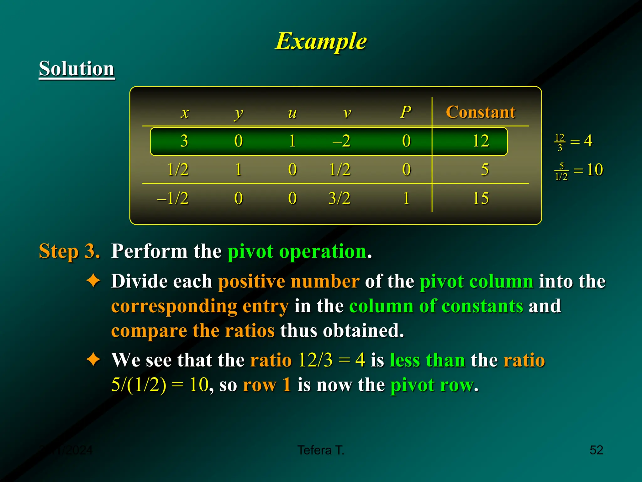
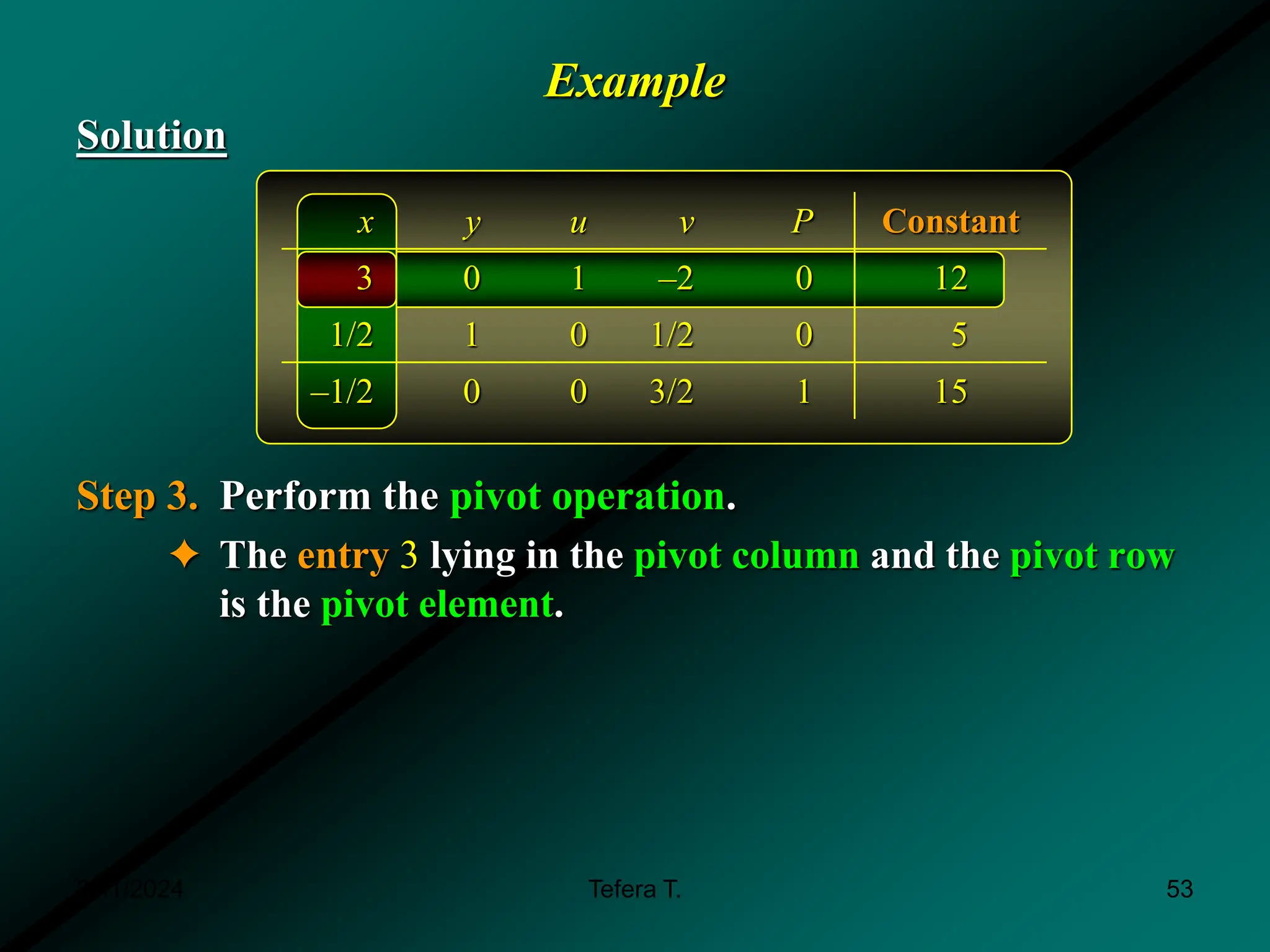
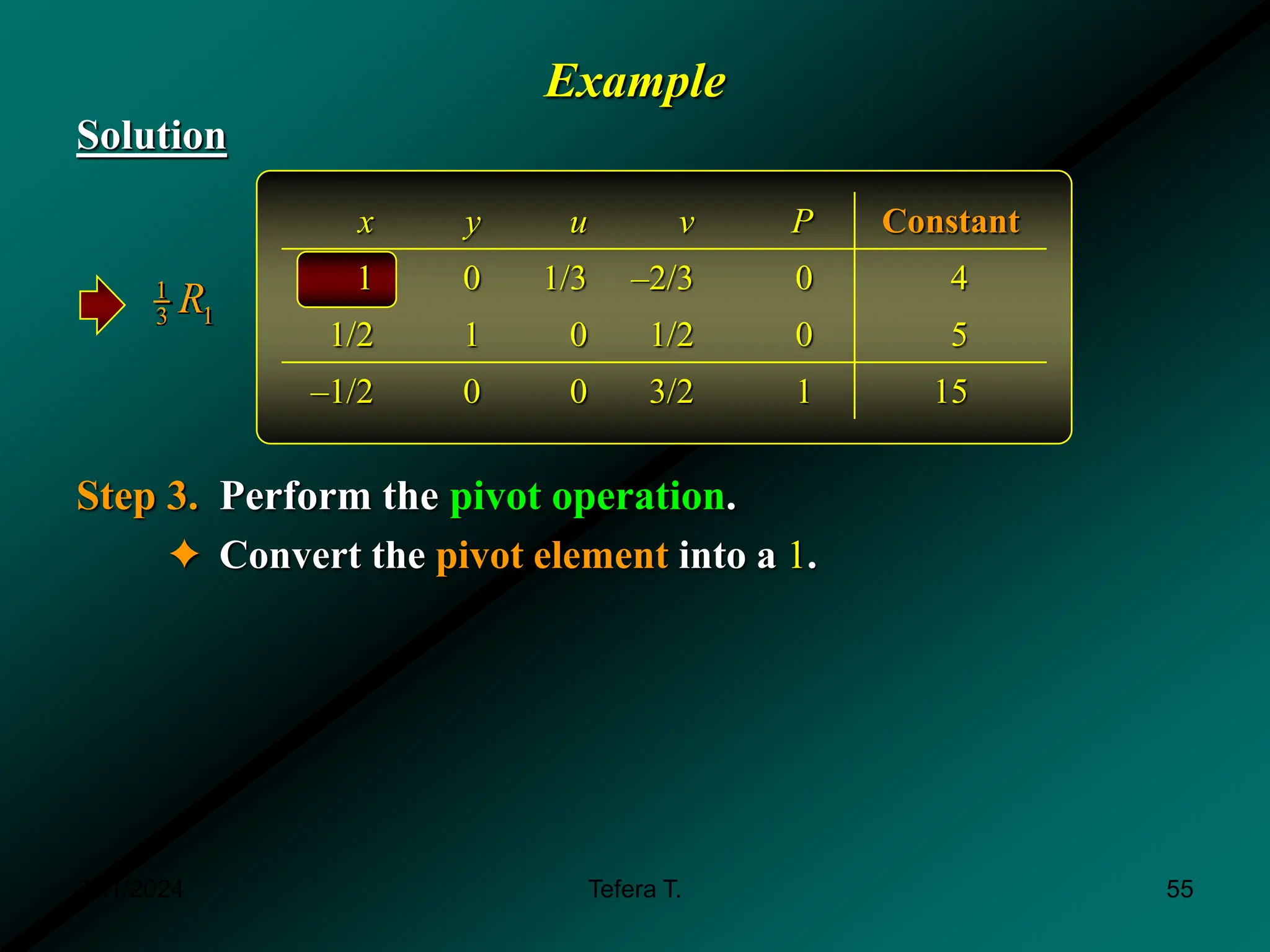
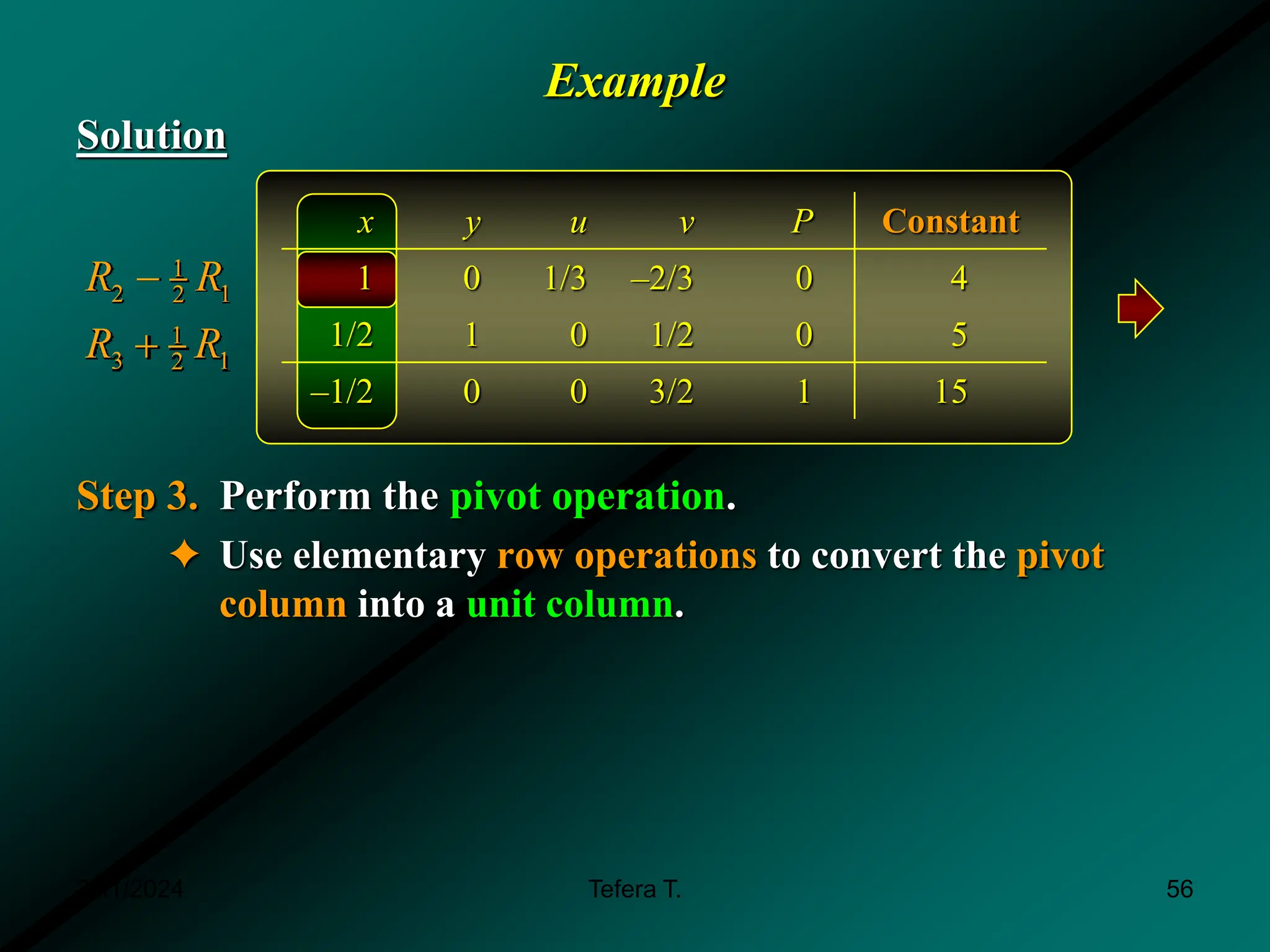
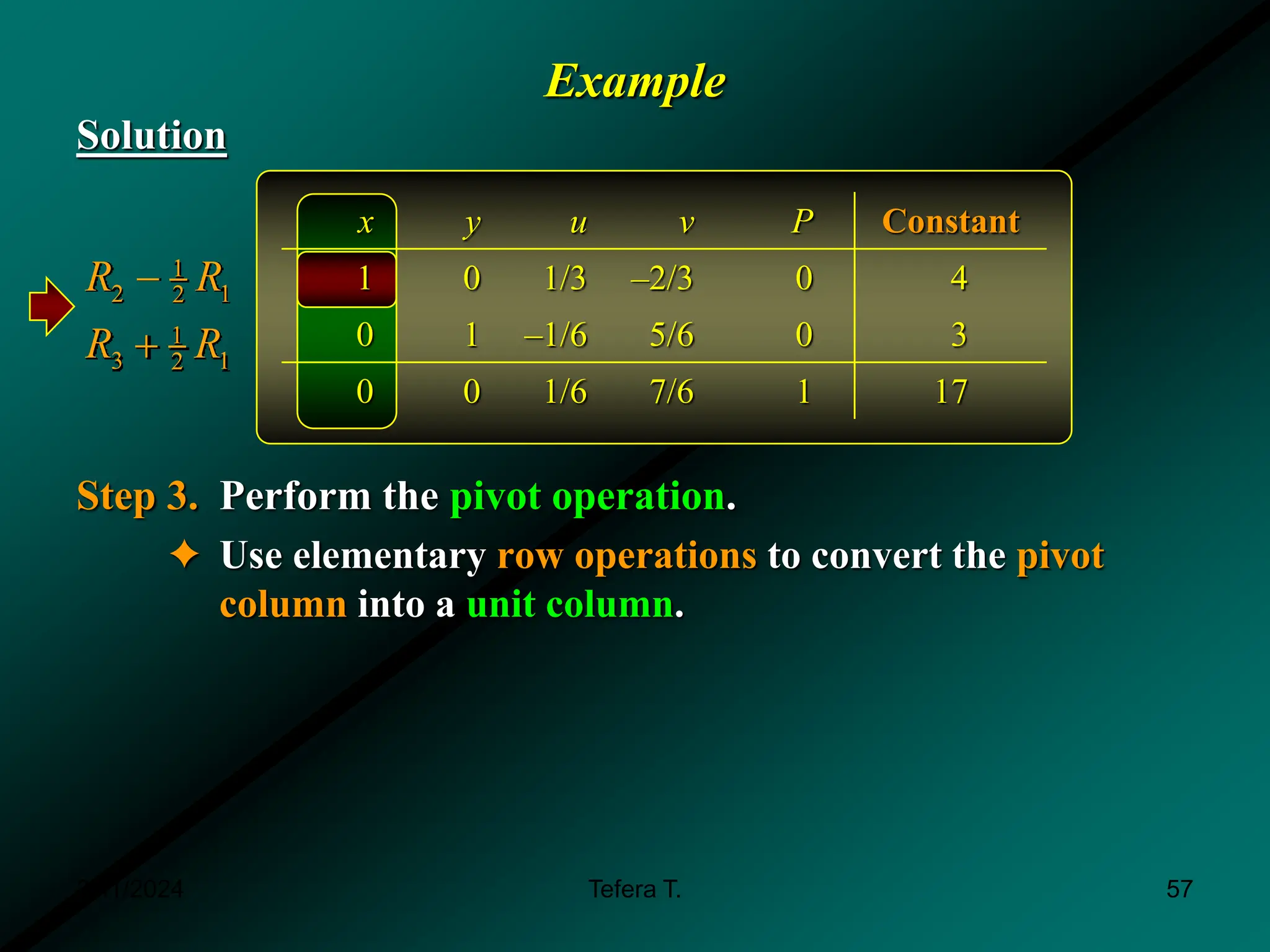
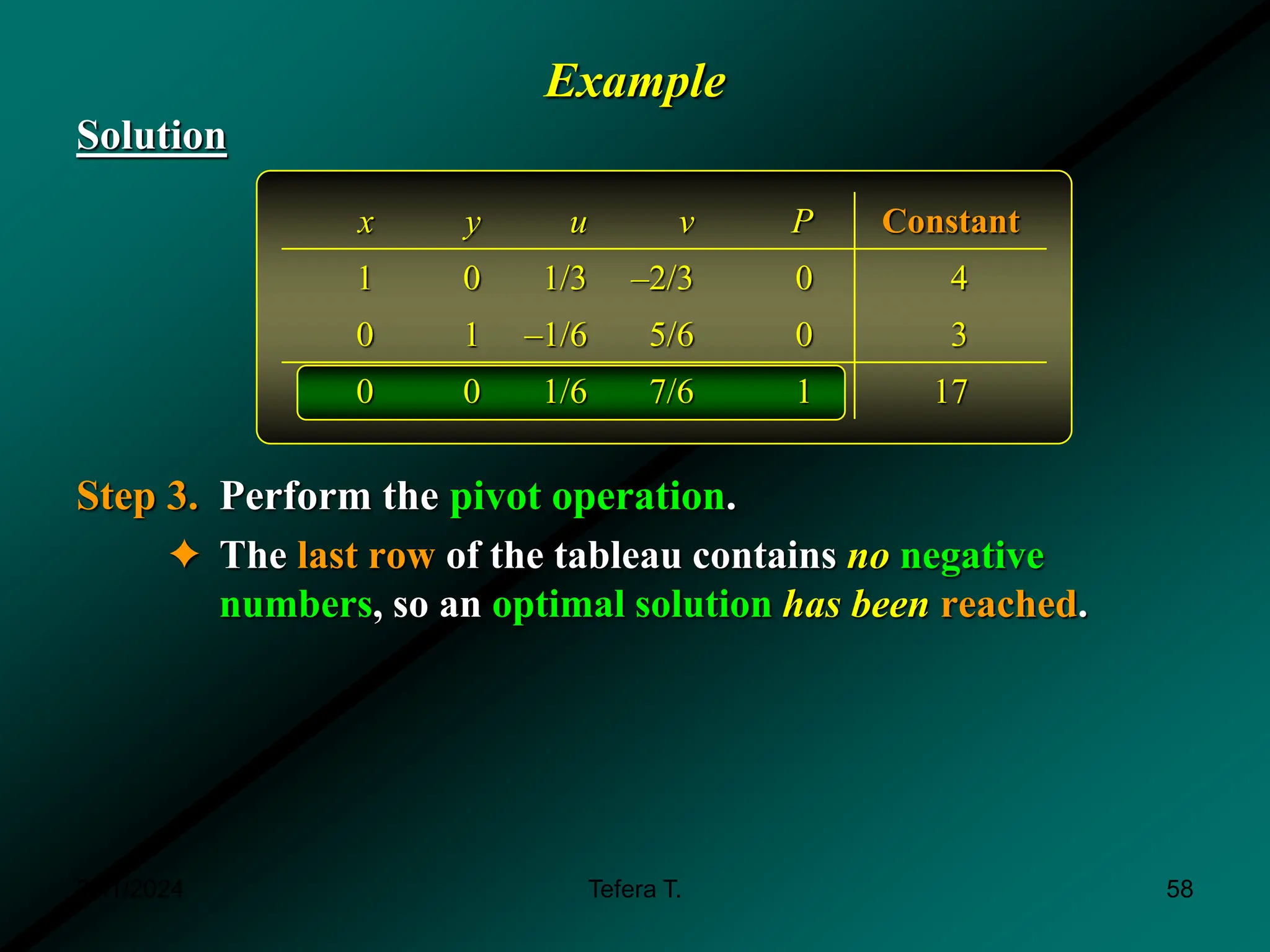
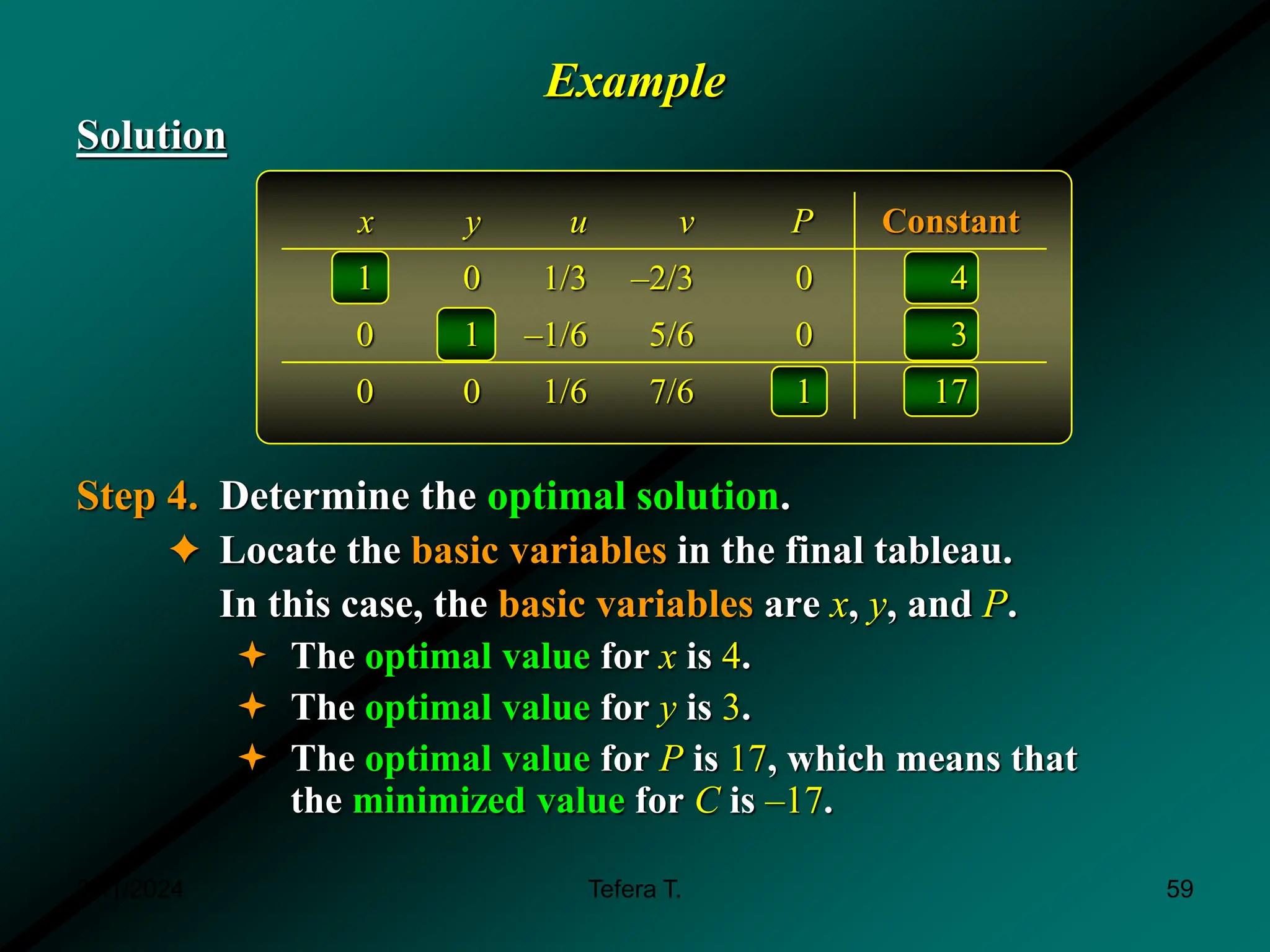
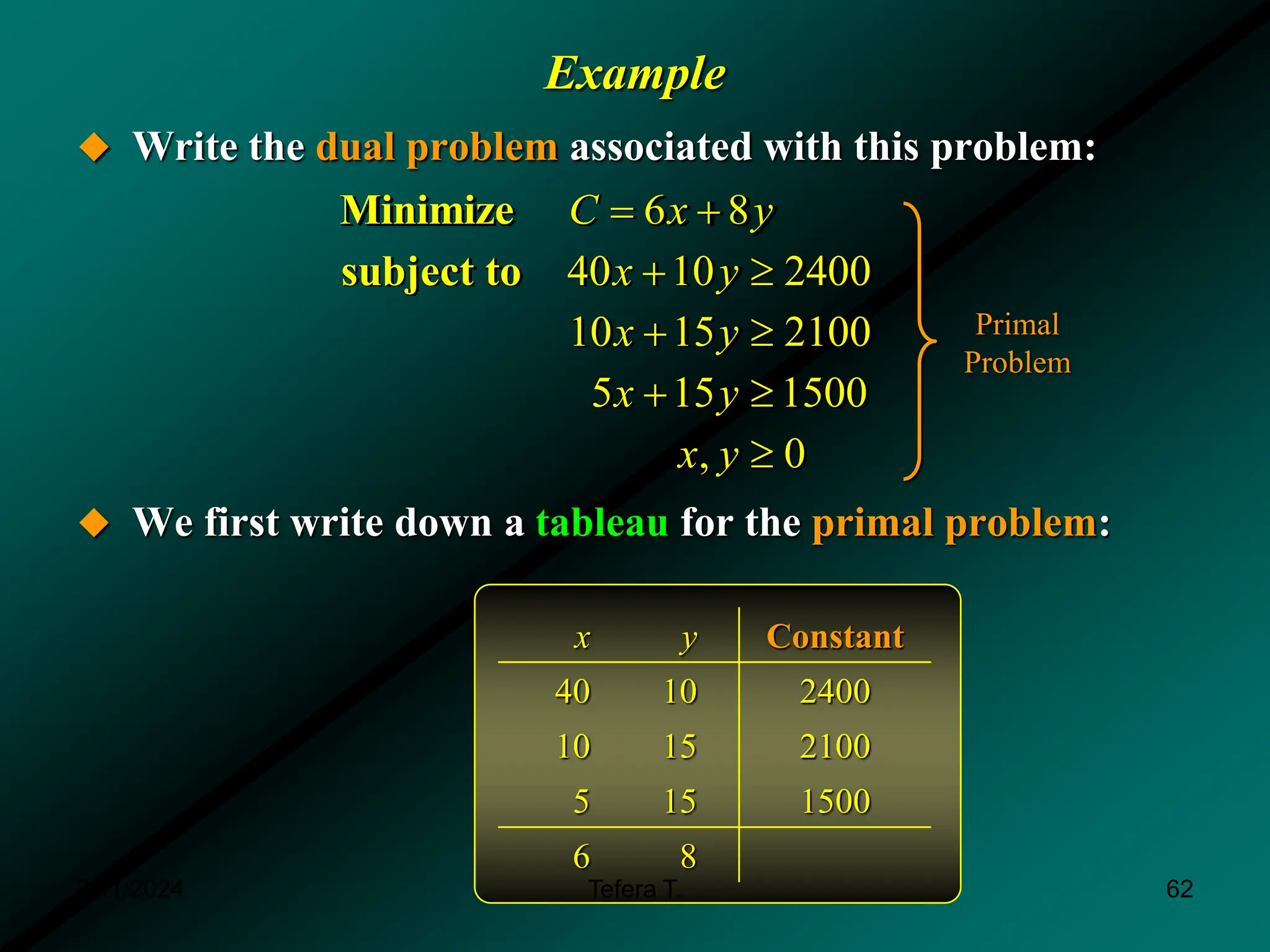
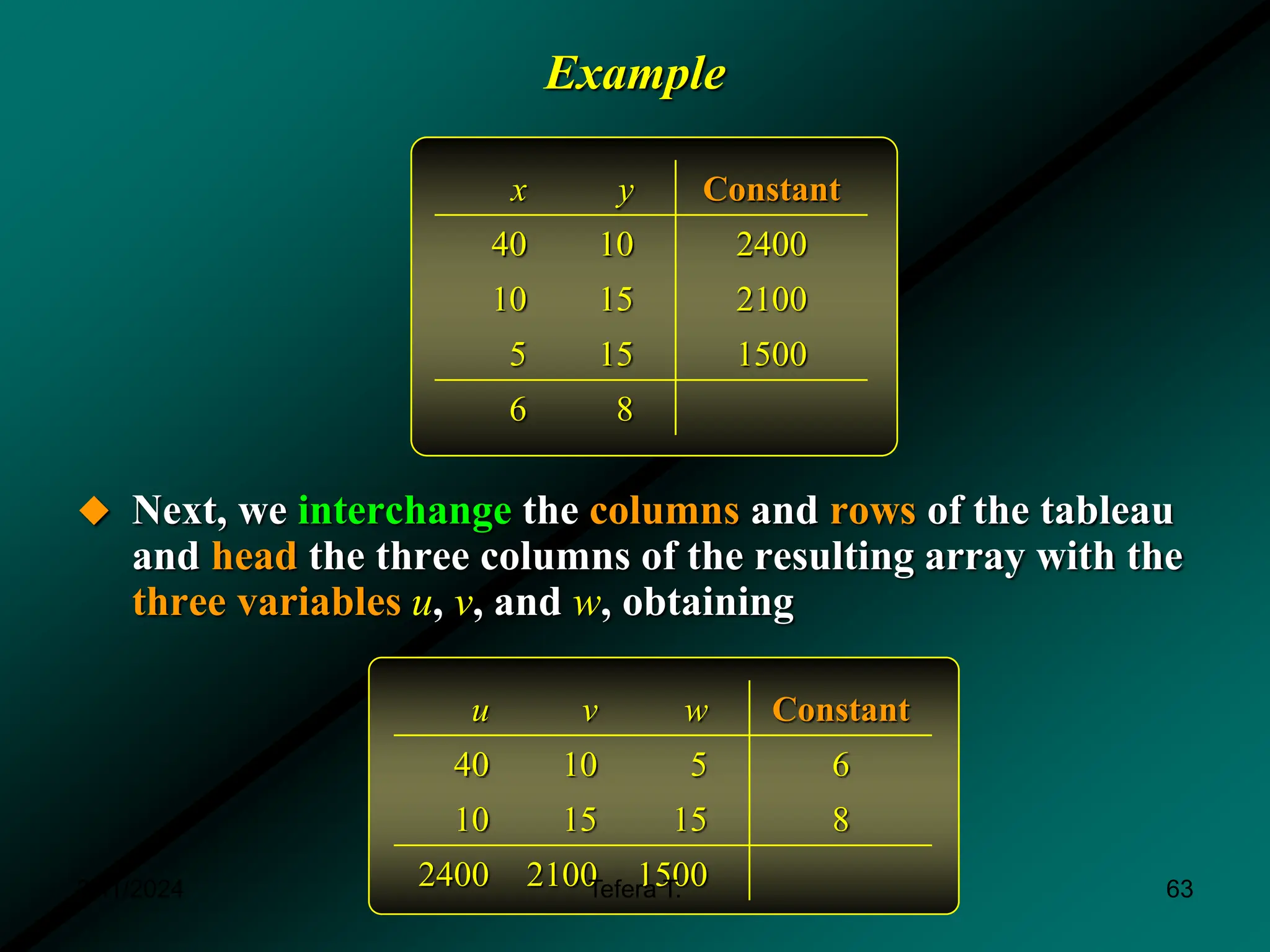
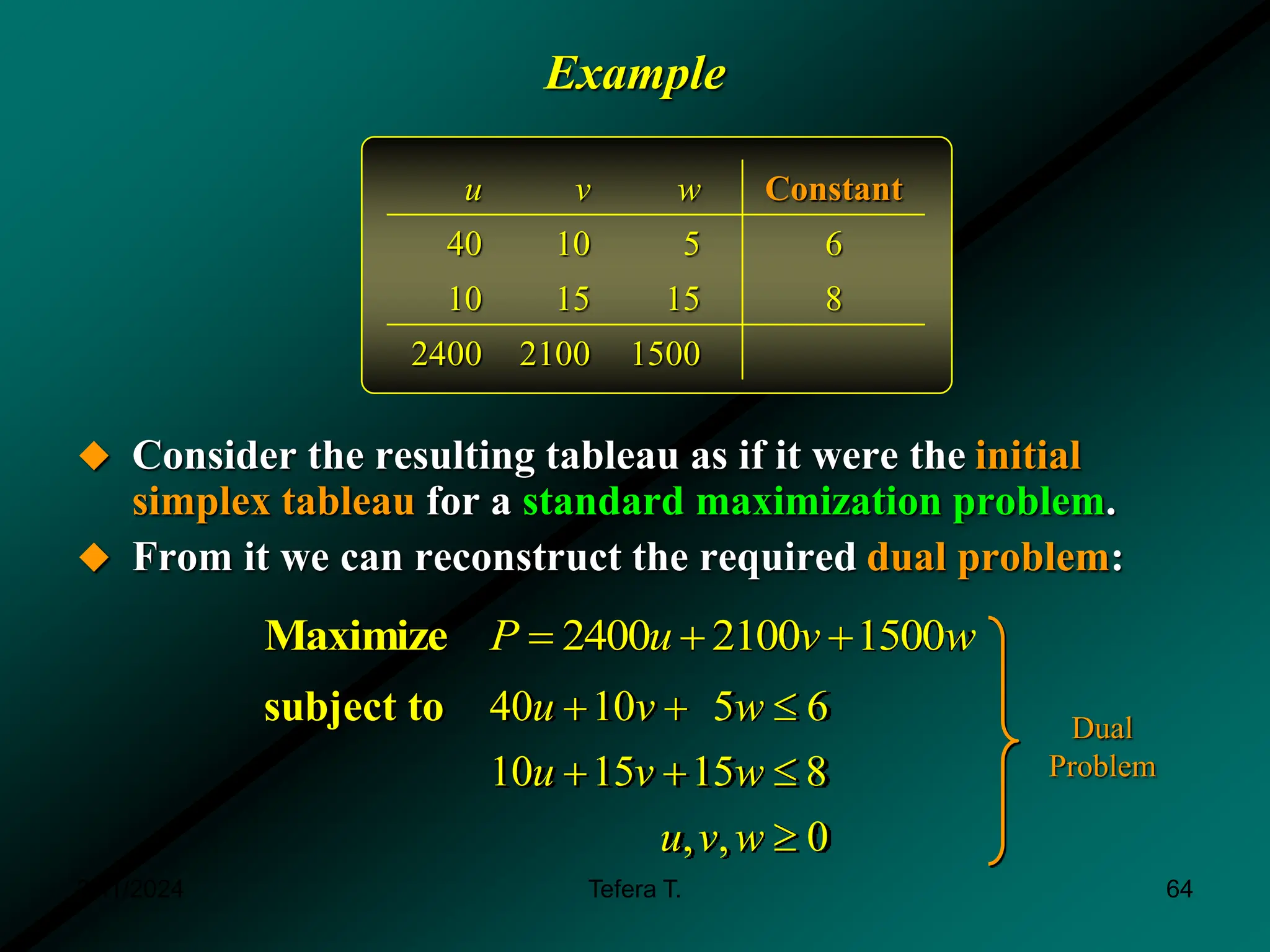
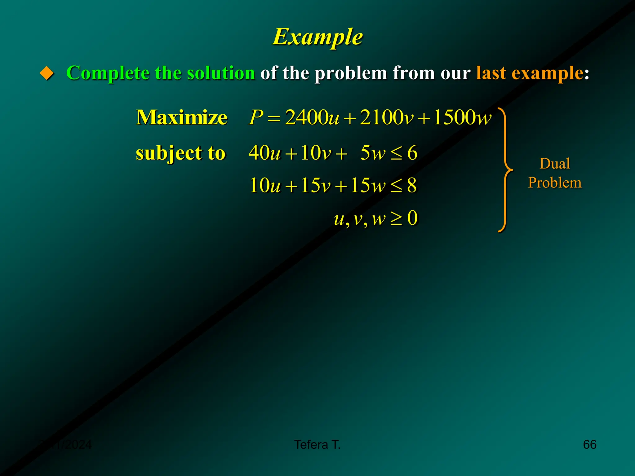
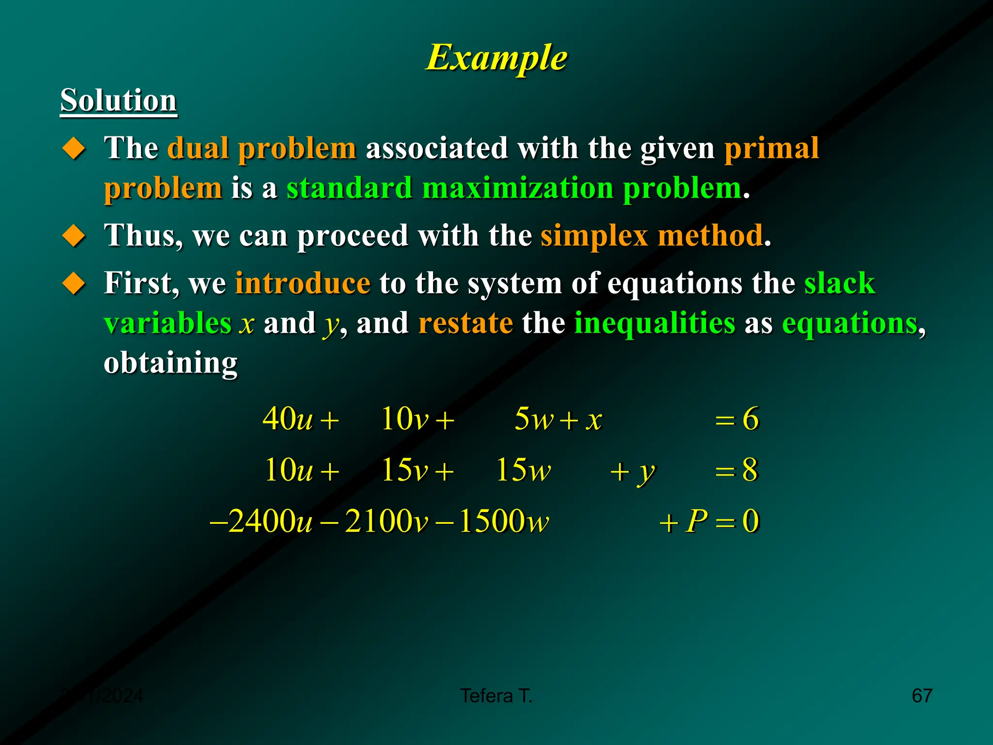
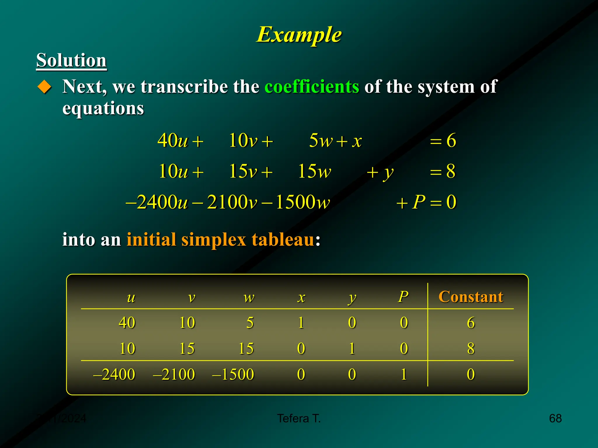
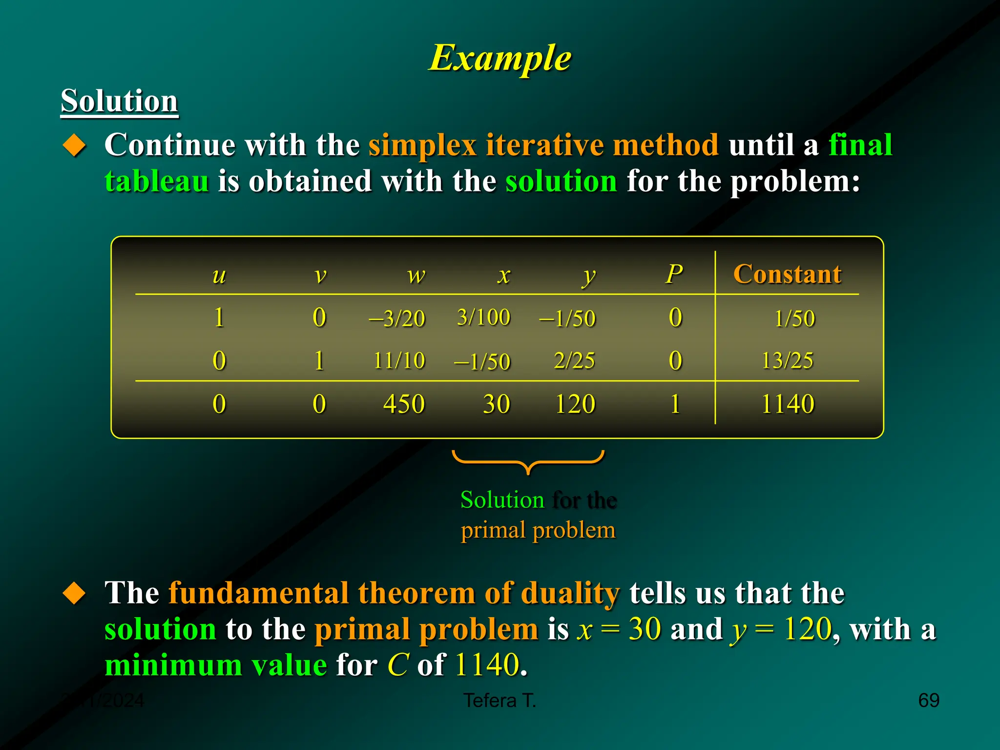
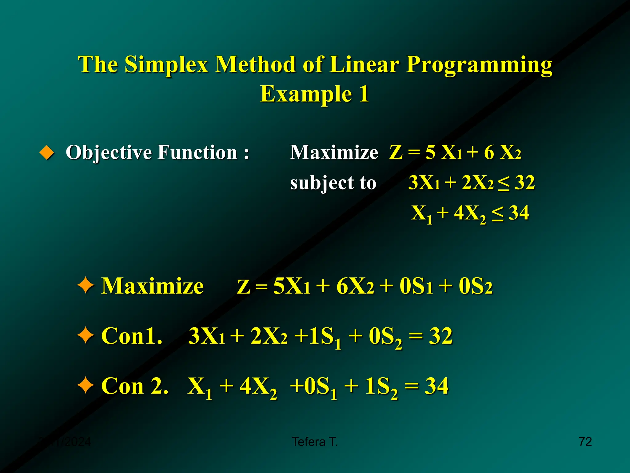
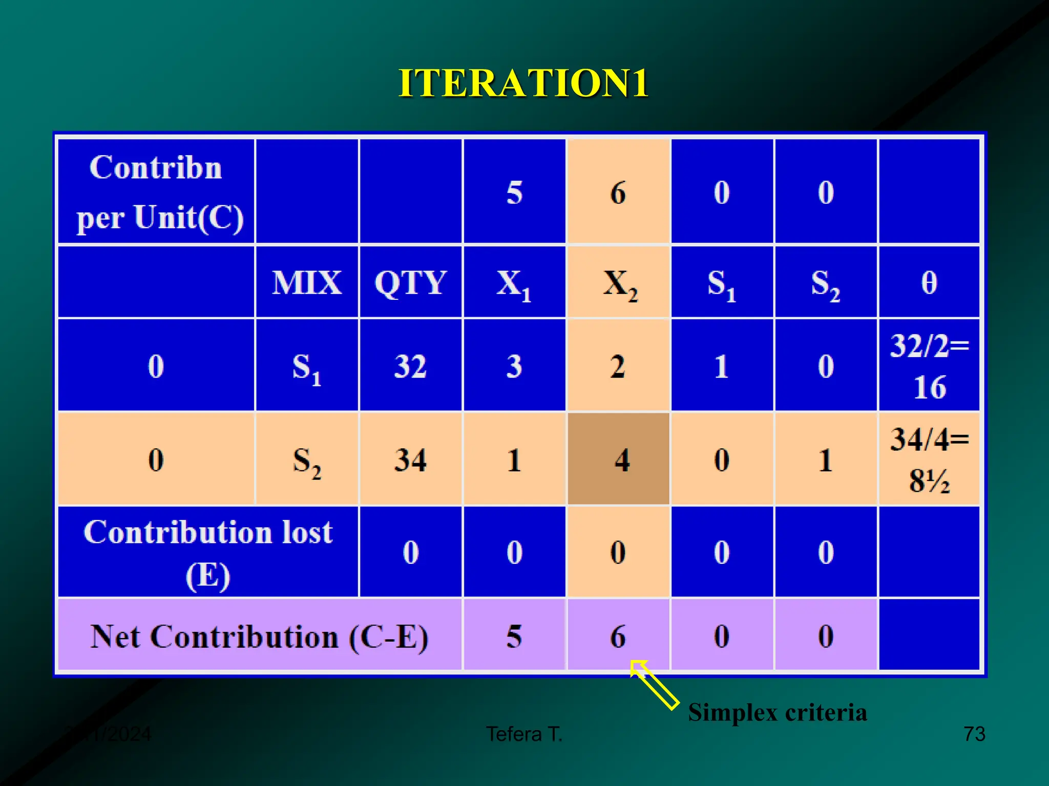
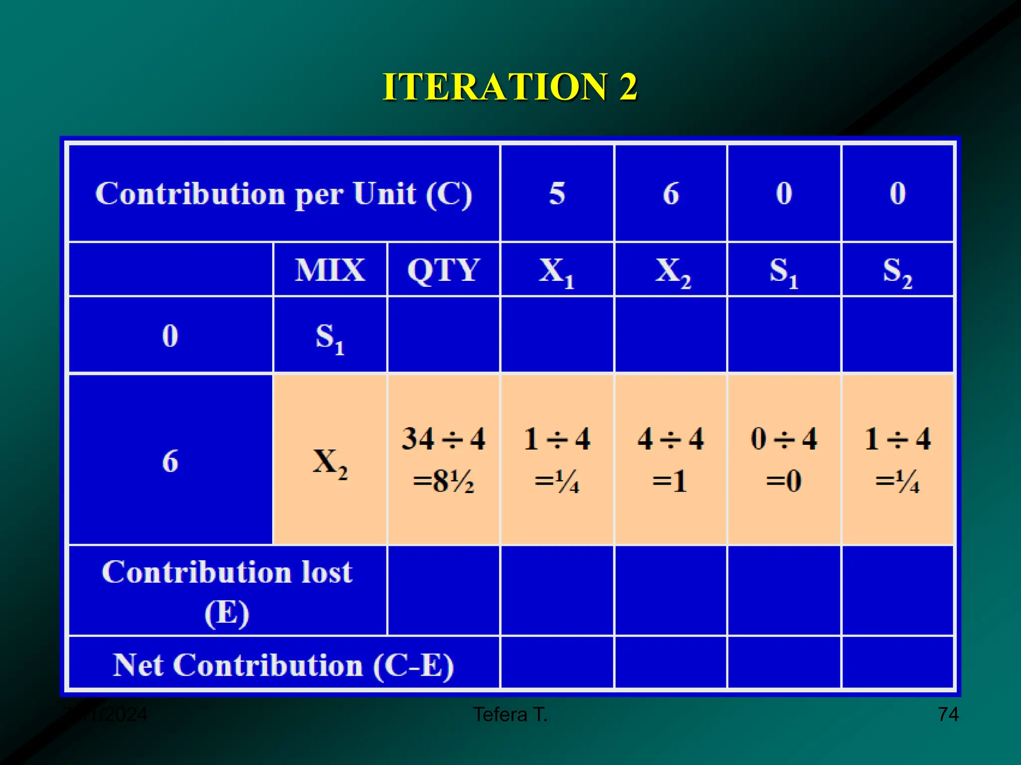
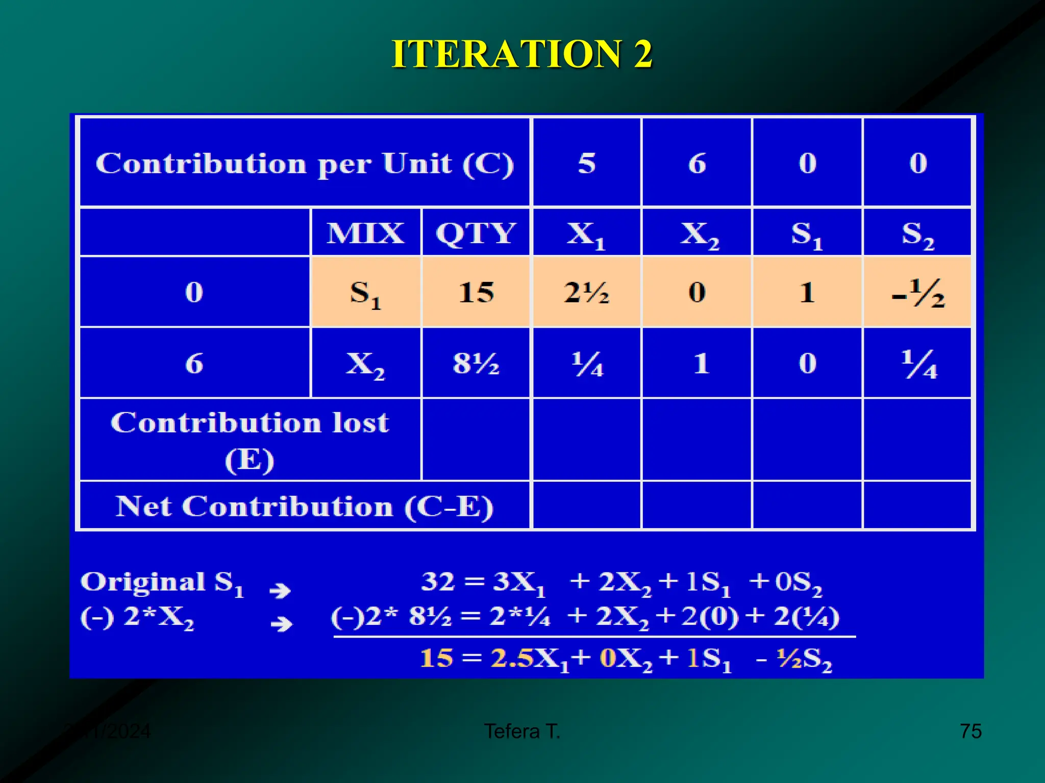
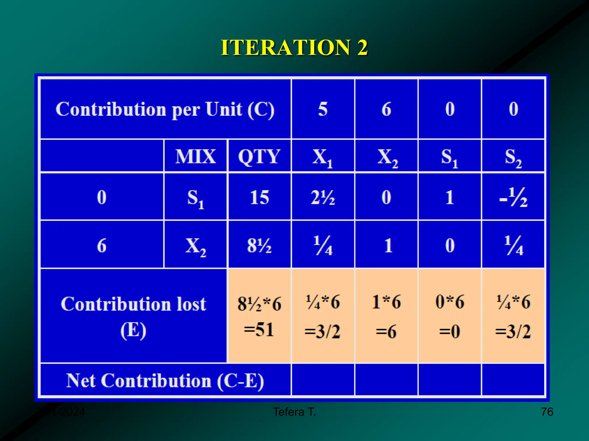
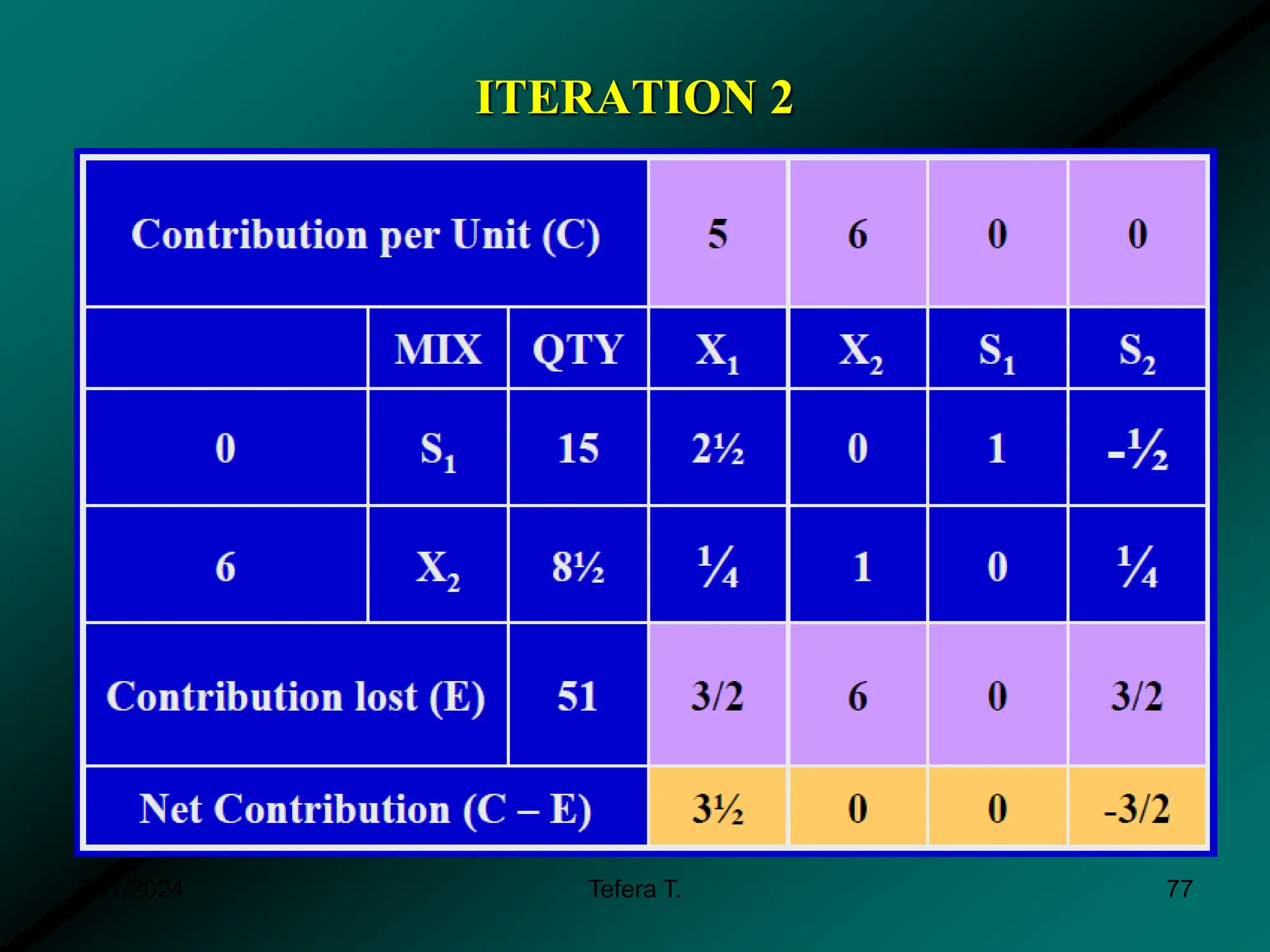
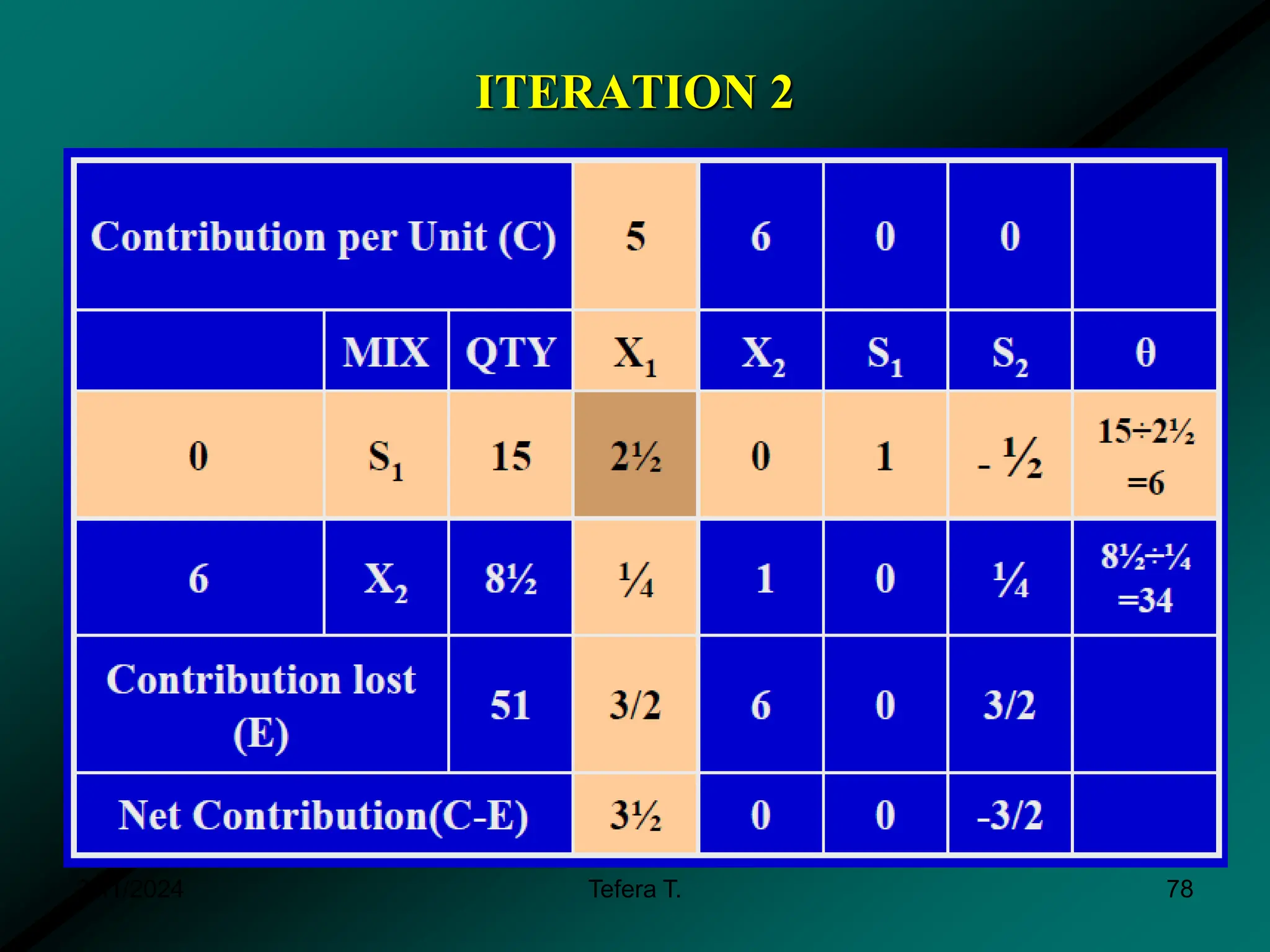
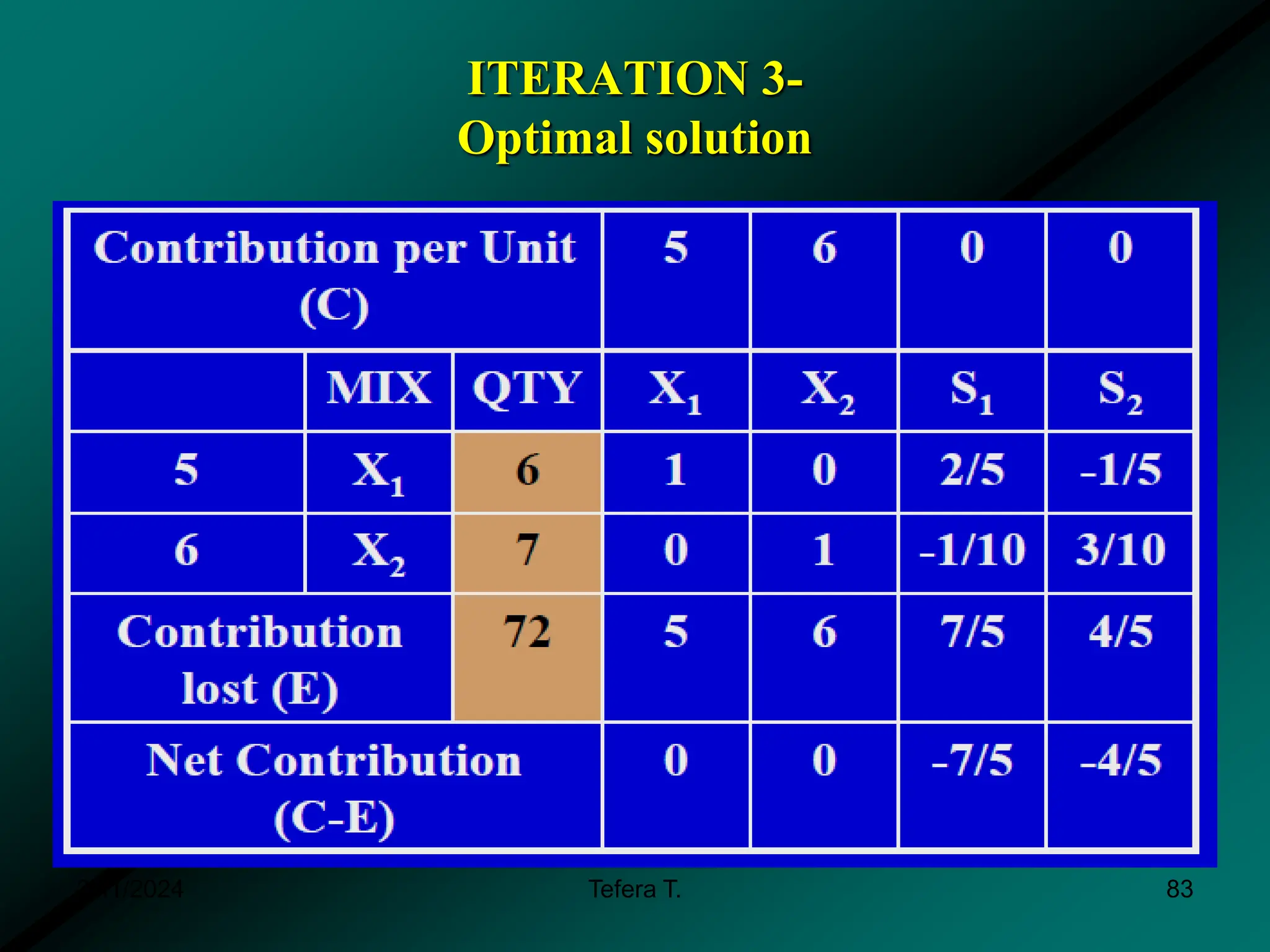
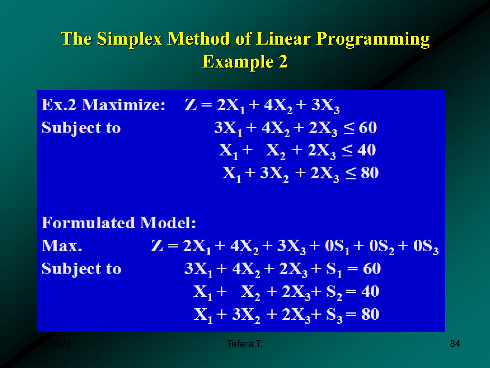
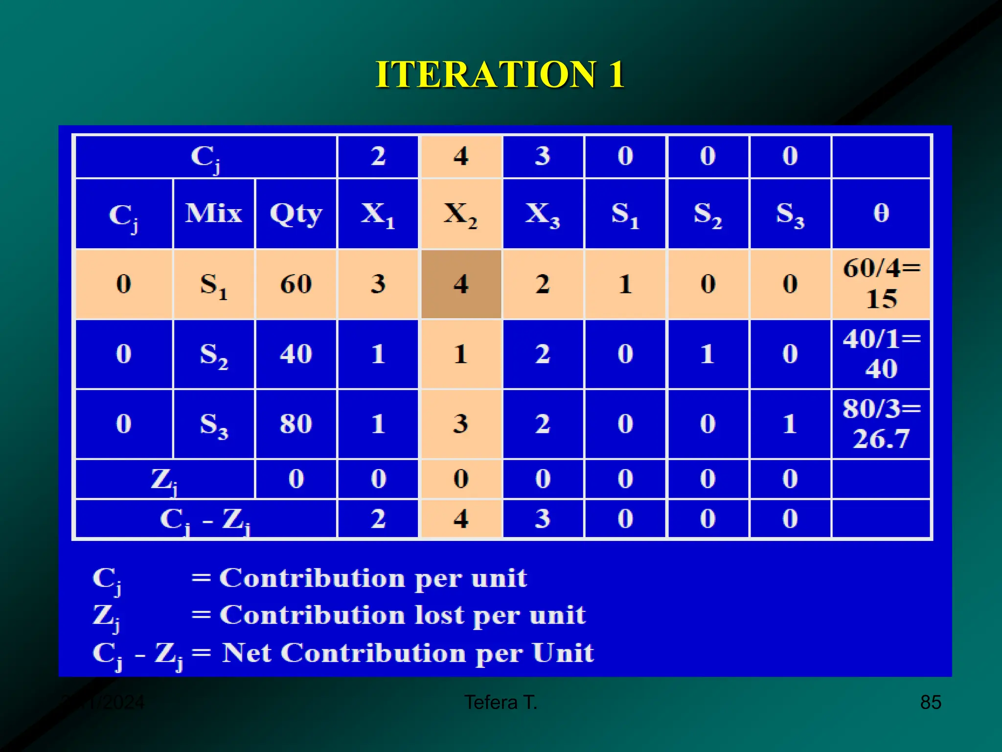
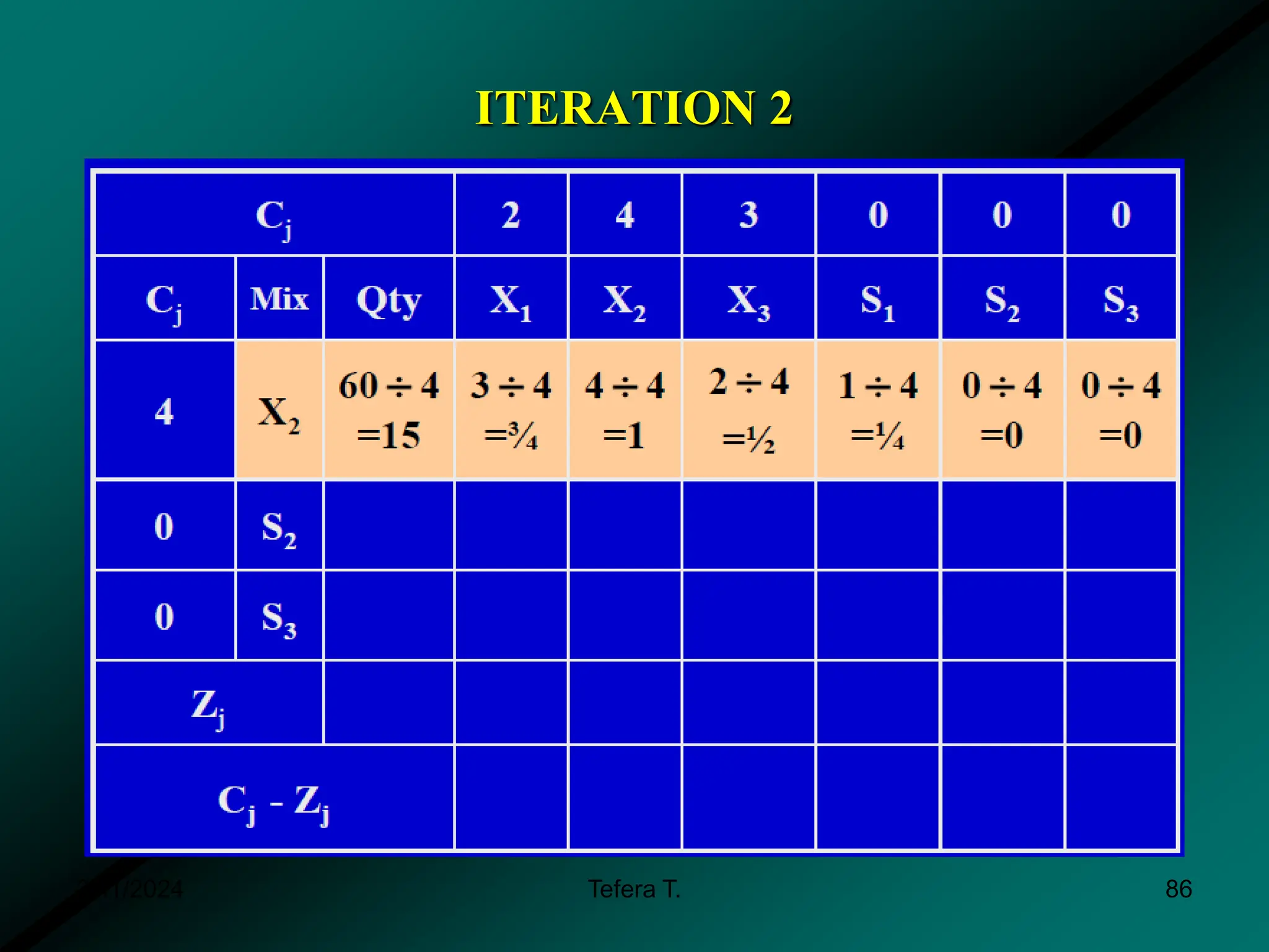
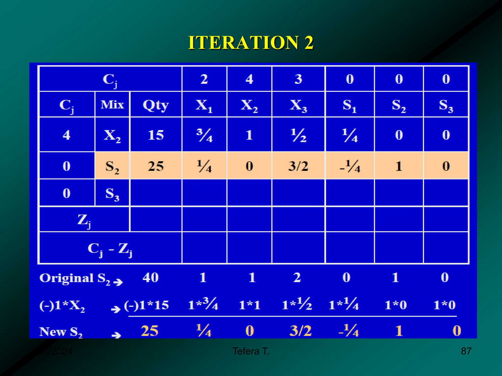
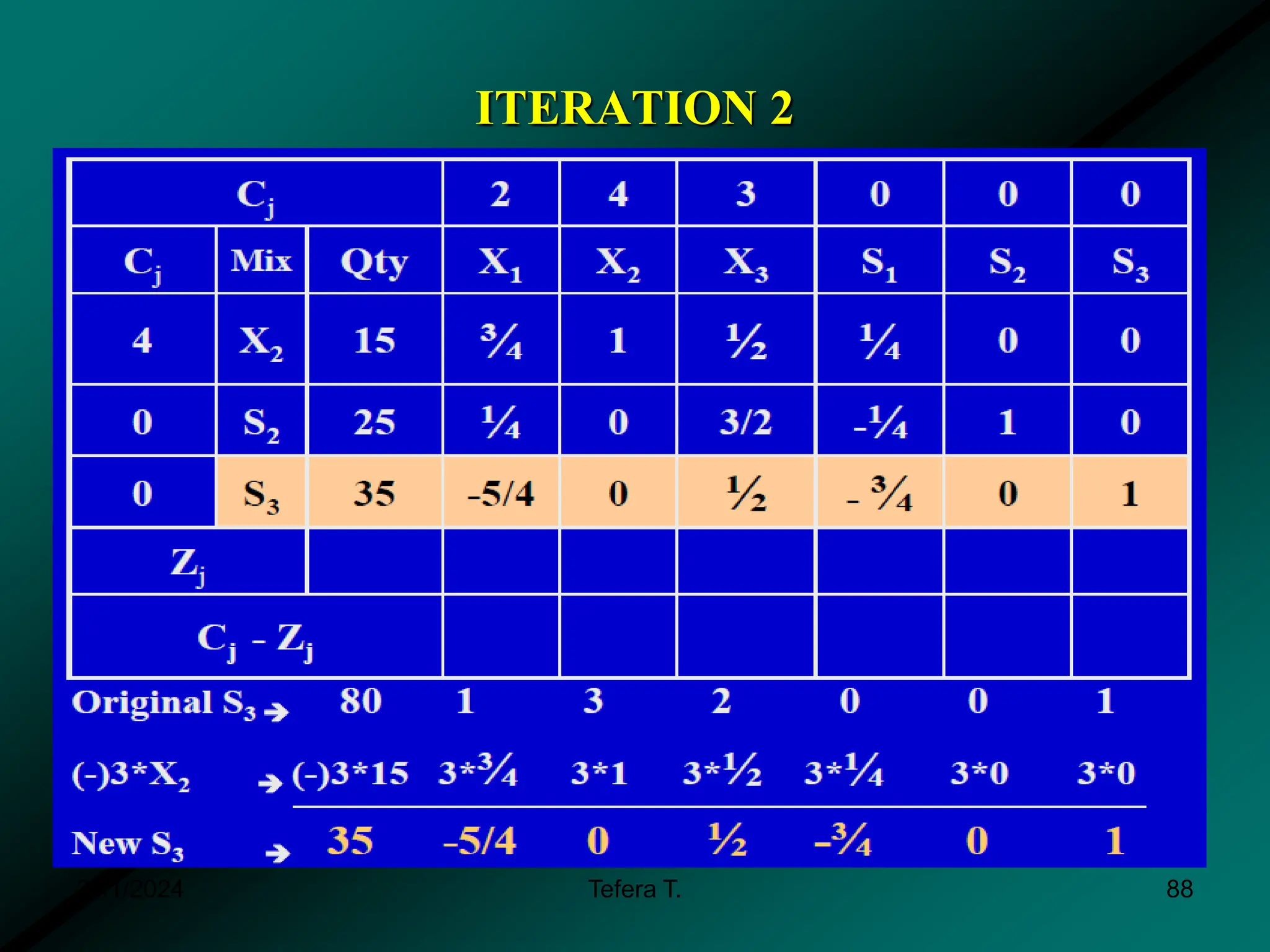
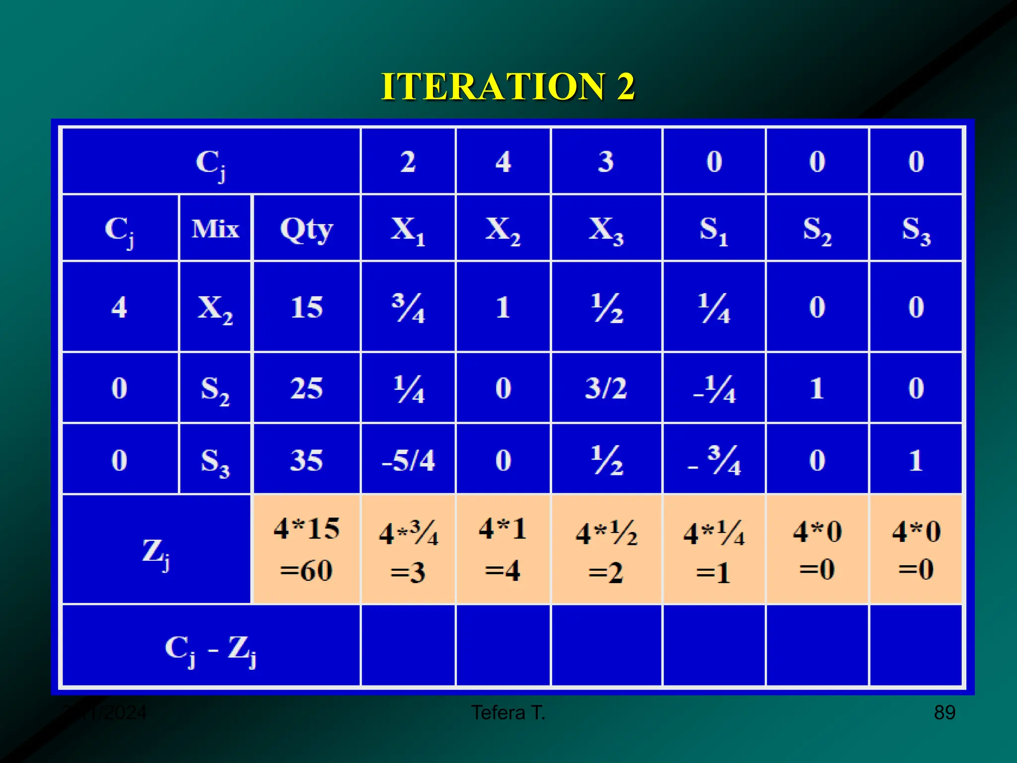
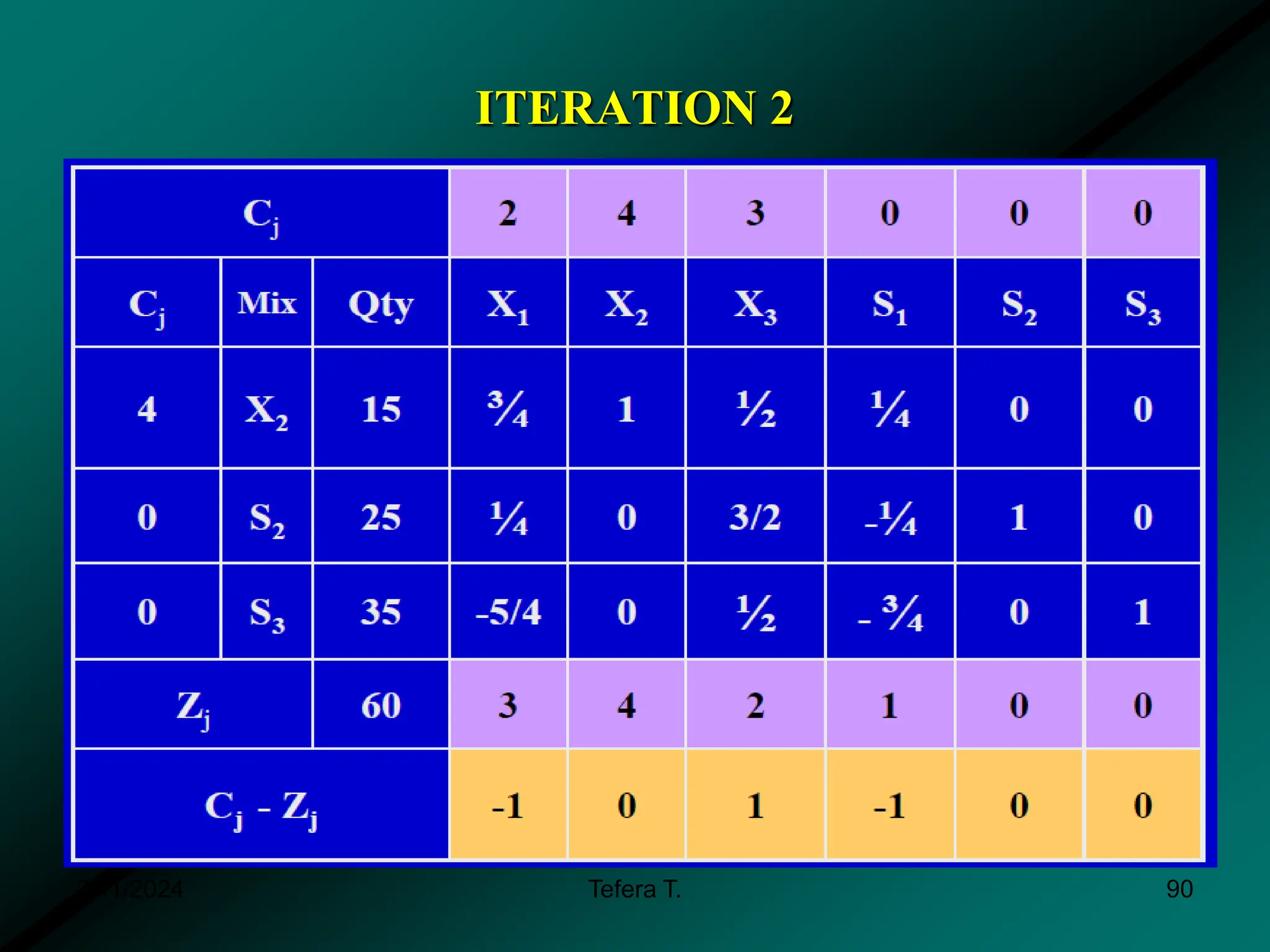
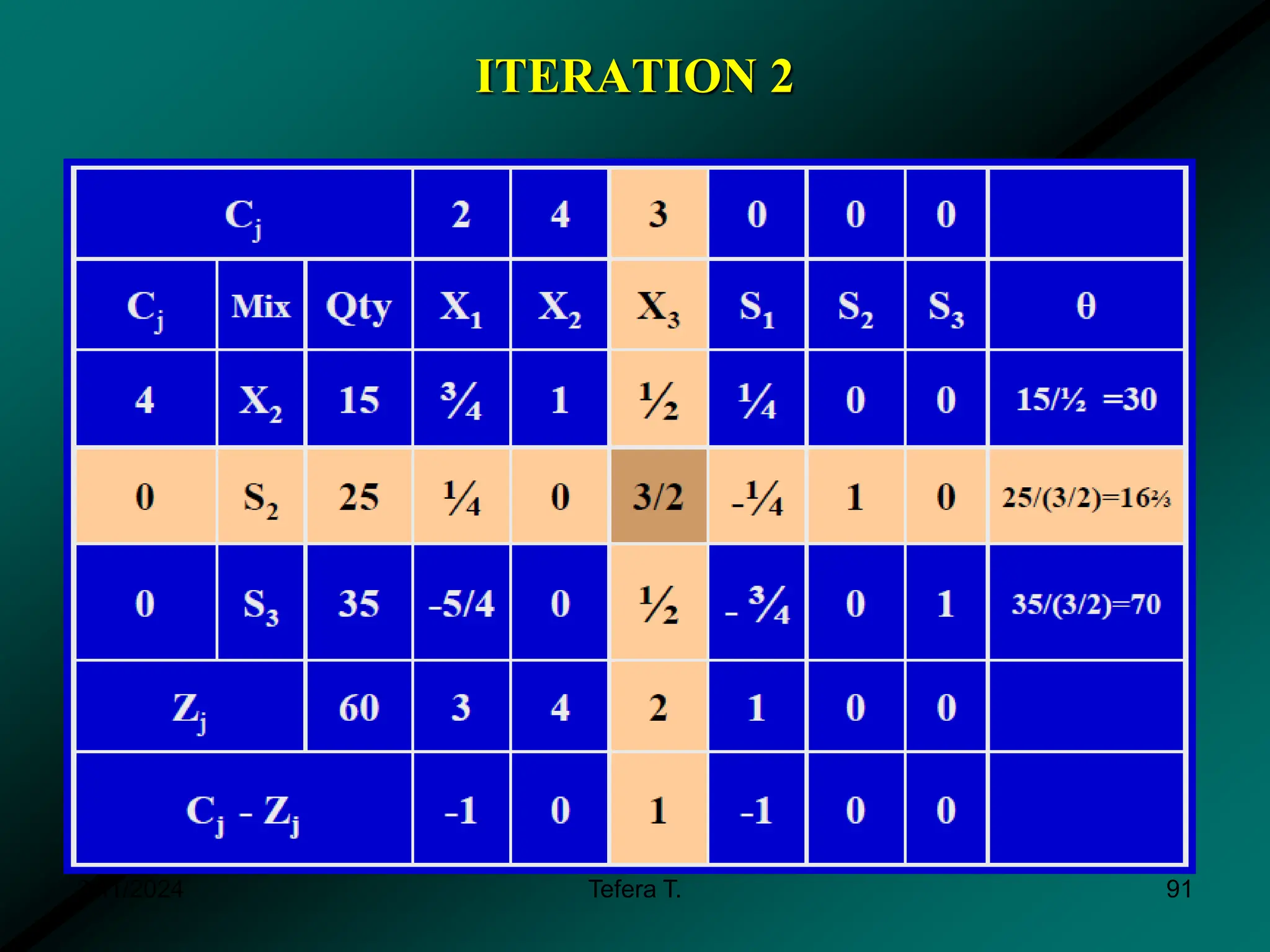
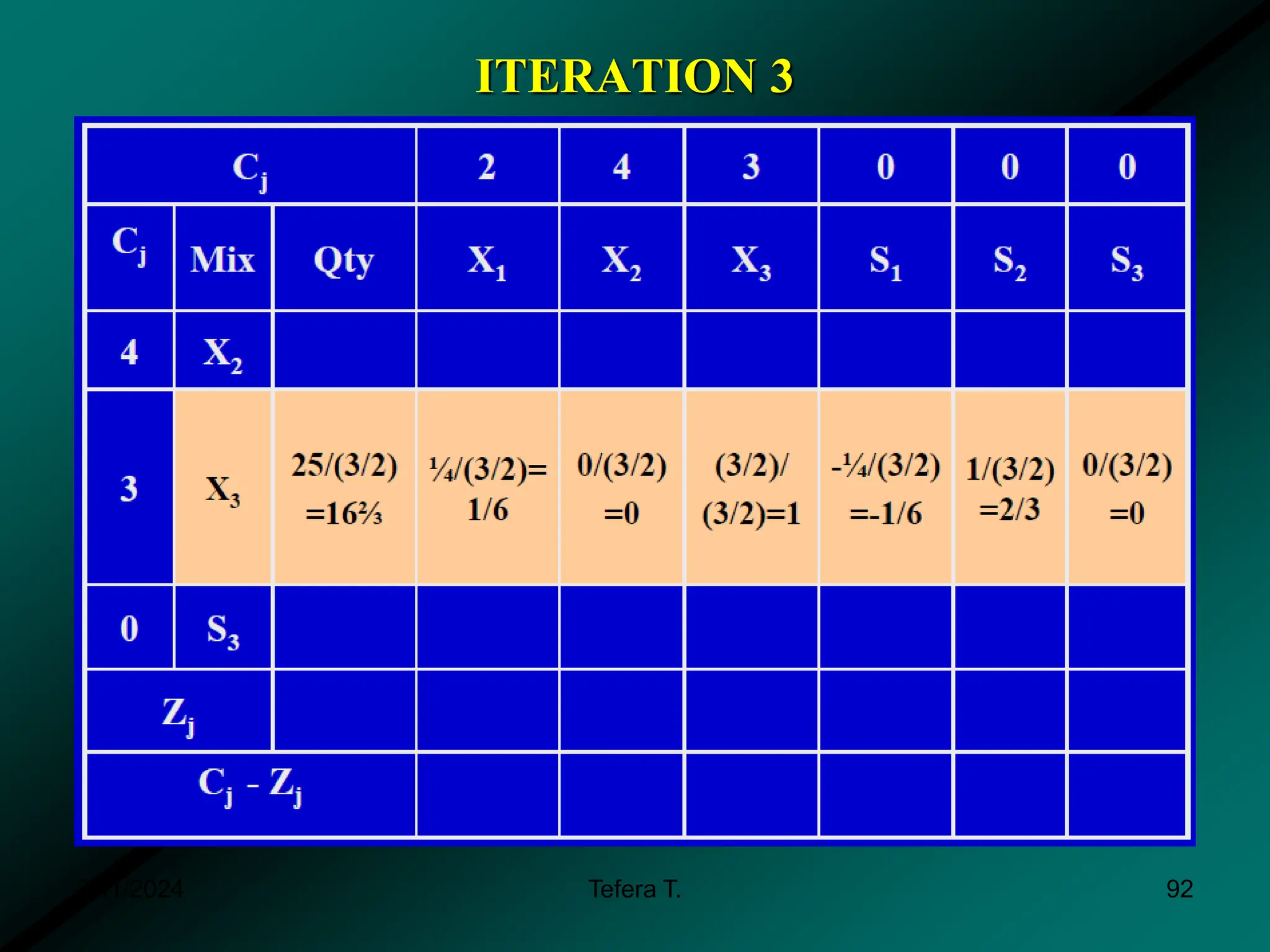
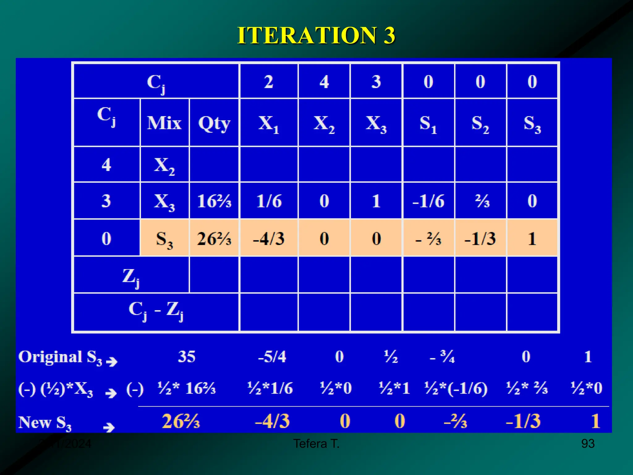
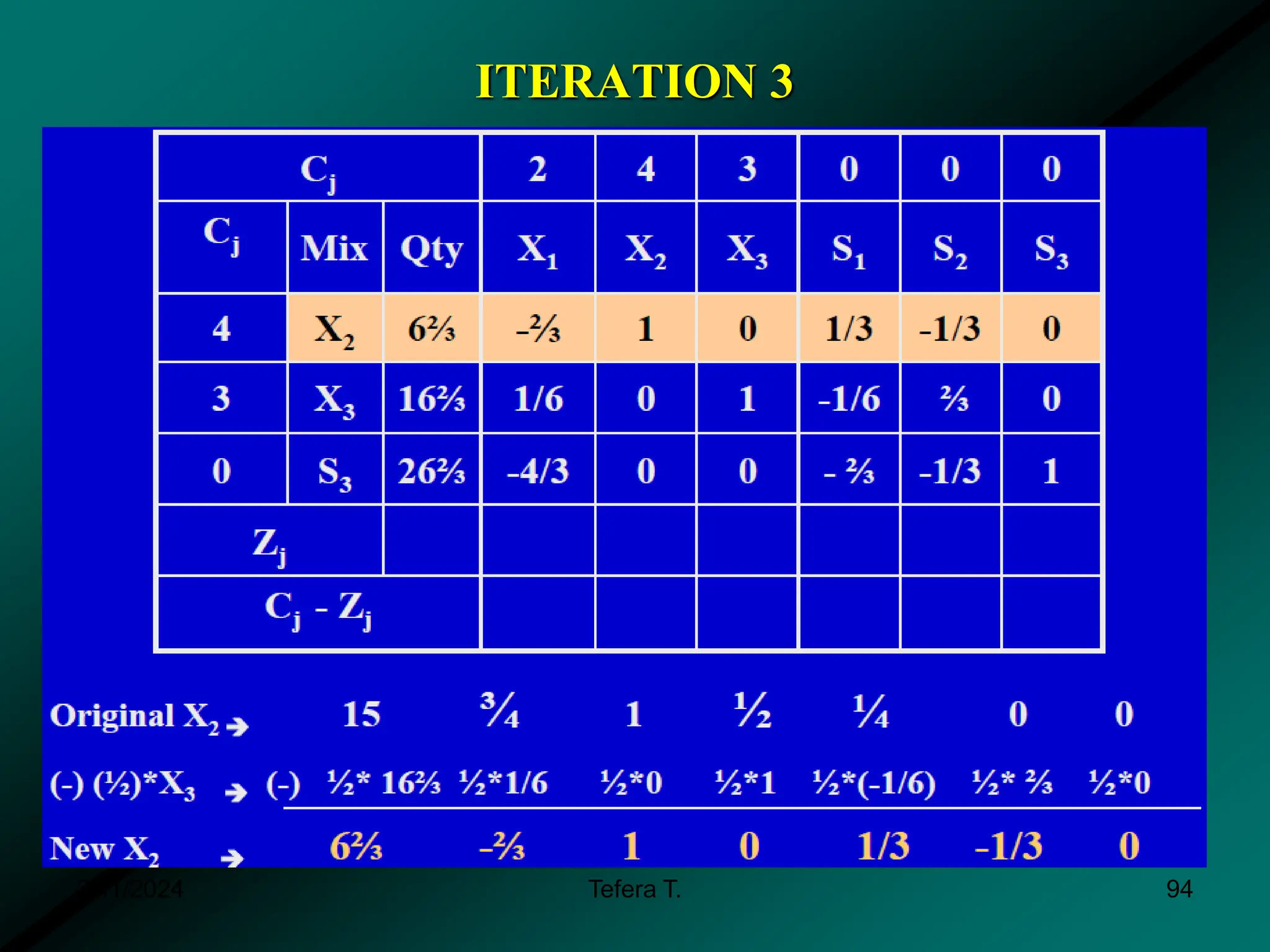
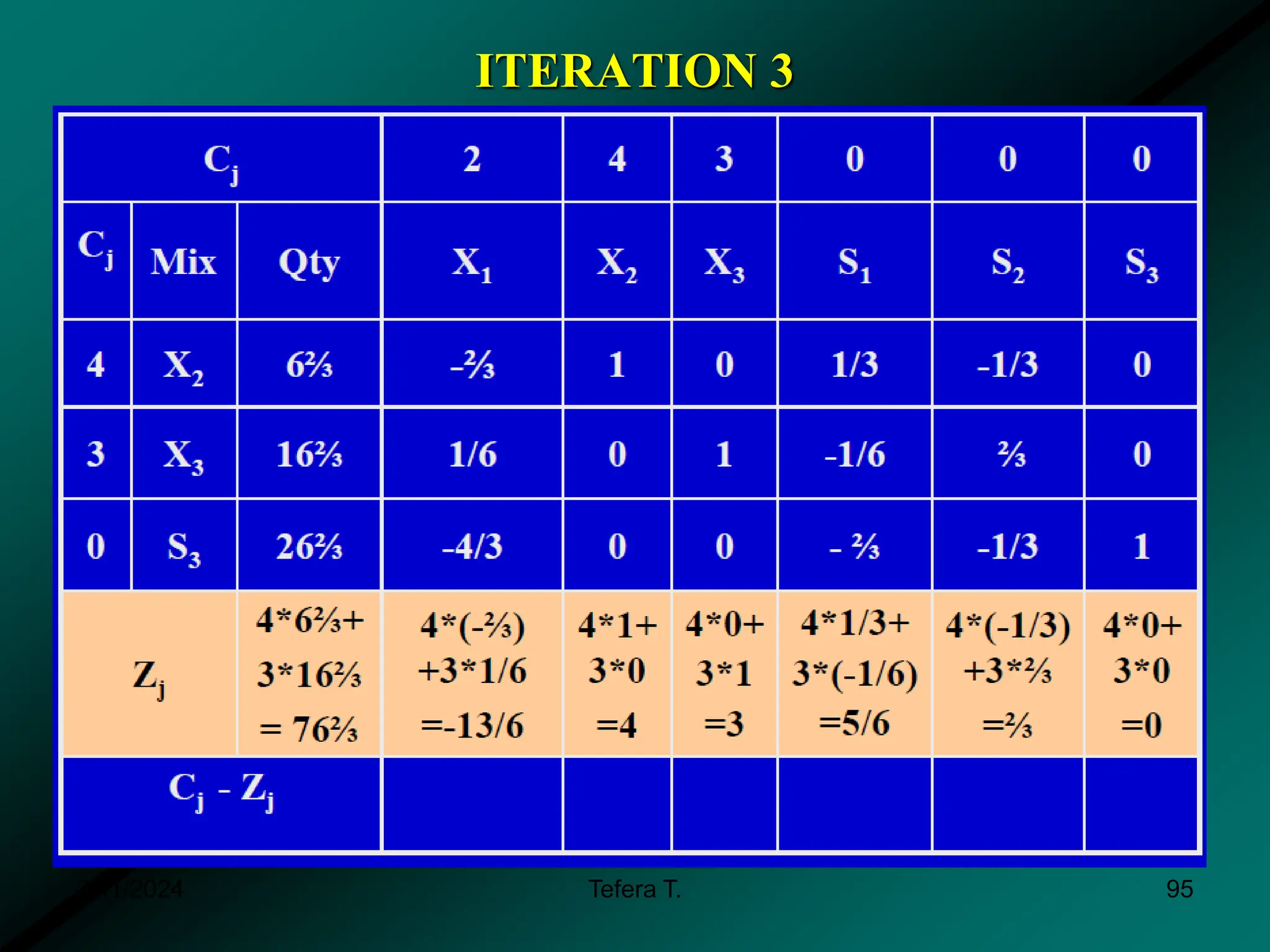
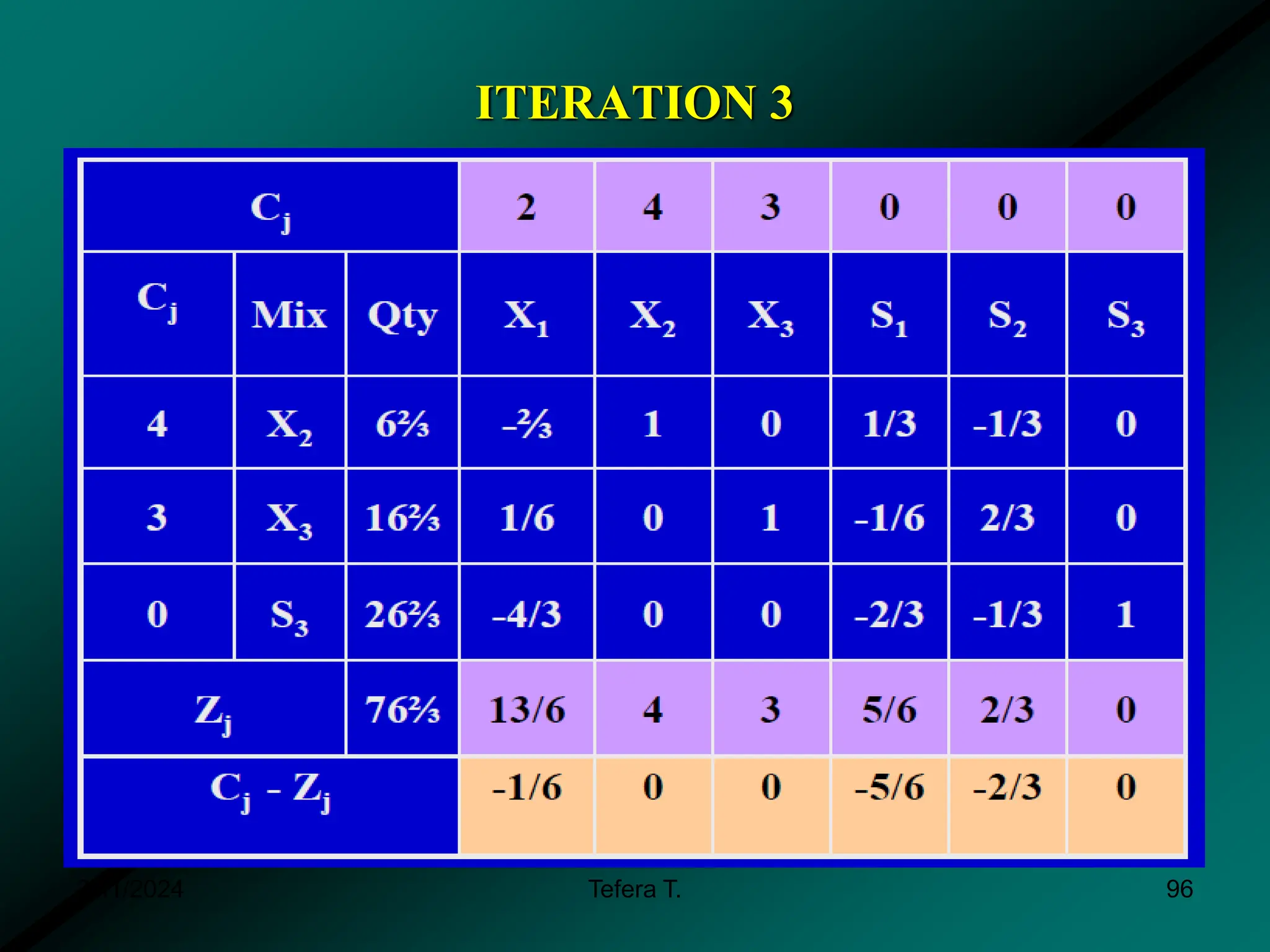
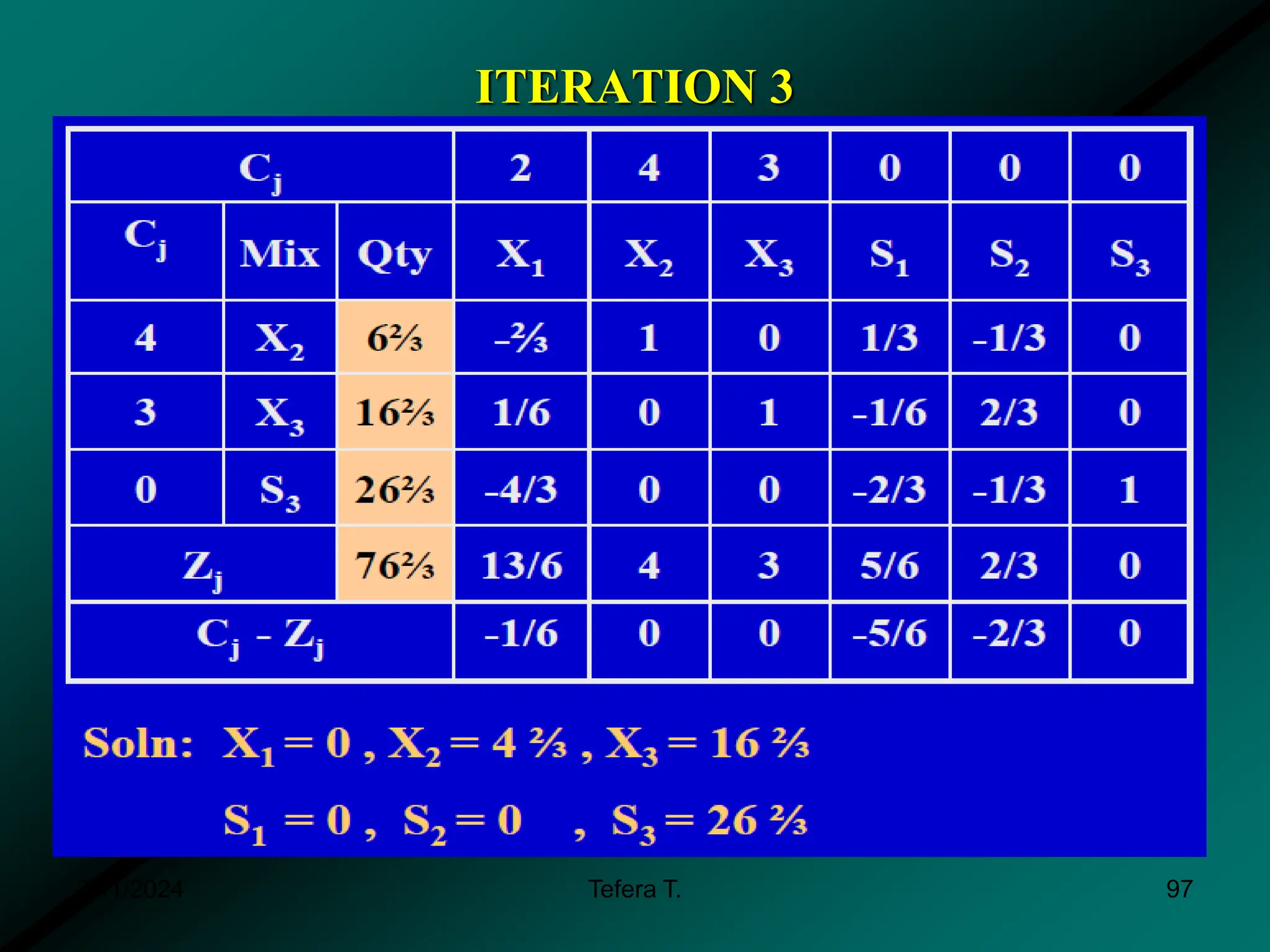
SlideShare a Scribd company logo
1 of 97
Linear Programming II : Simplex Algorithm
Chapter Three
✦ Introduction
✦ Simplex method
✦ Solution of maximization
problems
✦ Solution of minimization
problems
✦ Some special topics
3/11/2024 1
Tefera T.
The Simplex Method
 Simplex: a linear-programming algorithm that can solve
problems having more than two decision variables.
✦ The simplex technique involves generating a series of
solutions in tabular form, called tableaus.
✦ By inspecting the bottom row of each tableau, one can
immediately tell if it represents the optimal solution.
✦ Each tableau corresponds to a corner point of the feasible
solution space.
✦ The first tableau corresponds to the origin . Subsequent
tableaus are developed by shifting to an adjacent corner
point in the direction that yields the highest (smallest) rate
of profit (cost). This process continues as long as a positive
(negative) rate of cost (profit ) exists.
3/11/2024 2
Tefera T.
The key solution concepts in simplex
 Solution Concept 1: The simplex method focuses on CPF
solutions.
 Solution concept 2: The simplex method is an iterative
algorithm (a systematic solution procedure that keeps
repeating a fixed series of steps, called, an iteration, until a
desired result has been obtained) with the following
structure:
 Solution concept 3: Whenever possible, the initialization of
the simplex method chooses the origin point (all decision
variables equal zero) to be the initial CPF solution.
3/11/2024 Tefera T. 3
Simplex algorithm
3/11/2024 Tefera T. 4
Initialization: Setup to start iterations, including
finding an initial CPF solution.
Optimality test: is the current CPF solution
optimal?
if no if yes stop
Iteration: Perform an iteration to find a
better CFP solution
Simplex algorithm
 Solution concept 4: Given a CPF solution, it is much
quicker computationally to gather information about its
adjacent CPF solutions than about other CPF solutions.
✦ Therefore, each time the simplex method performs an
iteration to move from the current CPF solution to a better
one, it always chooses a CPF solution that is adjacent to the
current one.
 Solution concept 5: After the current CPF solution is
identified, the simplex method examines each of the edges of
the feasible region that emanate from this CPF solution.
✦ Each of these edges leads to an adjacent CPF solution at the
other end, but the simplex method doesn’t even take the
time to solve for the adjacent CPF solution.
3/11/2024 Tefera T. 5
Procedure for handling Constraints
3/11/2024 Tefera T. 7
Cont..
3/11/2024 Tefera T. 8
Test for optimality:
Case 1: Maximization problem
 The current BF solution is optimal if the last row is
negative.(<=0)
Case 2: Minimization problem
The current BF solution is optimal if the last row is
positive.(>=0)
1. New pivot row = old pivot row  pivot number
2. For the other row apply this rule:
New row = old row – the coefficient of this row in the
pivot column*(new pivot row).
The Simplex Method of Linear Programming
Steps
 Express the objective function as an
equation.
 Set up the Constraint inequalities.
 Convert the inequalities to equations by
adding slack variables.
 Finally, add zero value variables so that all
variables appear in all equations.
3/11/2024 Tefera T. 9
Simplex Method
3/11/2024 Tefera T. 10
A. Qty. of each Variable
B. List of all Variables
C. Contribution per Unit of each Variable in Profit Equation
D. Relationship
E. Accounting for Transaction
3/11/2024 Tefera T. 11
The Simplex Method:
Standard maximization Problems
A Standard Linear Programming Problem
 A standard maximization problem is one in
which
1. The objective function is to be maximized.
2. All the variables involved in the problem are
nonnegative.
3. All other linear constraints may be written so
that the expression involving the variables is less
than or equal to a nonnegative constant.
3/11/2024 12
Tefera T.
Setting Up the Initial Simplex Tableau
1. Transform the system of linear inequalities
into a system of linear equations by
introducing slack variables.
2. Rewrite the objective function
in the form
where all the variables are on the left and the
coefficient of P is +1. Write this equation
below the equations in step 1.
3. Write the augmented matrix associated with
this system of linear equations.
1 1 2 2 n n
P c x c x c x
  
1 1 2 2 0
n n
c x c x c x P
    
3/11/2024 13
Tefera T.
Applied Example 1: A Production Problem
 Recall the production problem discussed in chapter 1,
which required us to maximize the objective function
subject to the system of inequalities
 This is a standard maximization problem and may be
solved by the simplex method.
 Set up the initial simplex tableau for this linear
programming problem.
, 0
x y 
6
1.2
5
P x y P x y
   
or equivalently,
3 300
x y
 
2 180
x y
 
3/11/2024 14
Tefera T.
Applied Example 1: A Production Problem
Solution
 First, introduce the slack variables s1 and s2 into the
inequalities
and turn these into equations, getting
2x + y + s1 + 0s2 = 180
X + 3y + 0s1 + s2 = 300
 Next, rewrite the objective function in the form
3 300
x y
 
2 180
x y
 
6
0
5
x y P
   
3/11/2024 15
Tefera T.
Applied Example 1: A Production Problem
Solution
 Placing the restated objective function below the system of
equations of the constraints we get
2x + y + s1 + 0s2 = 180
X + 3y + 0s1 + s2 = 300
- x- 6/5y + 0s1 + 0s2 = 0
 Thus, the initial tableau associated with this system is
x y s1 s2 P Constant
2 1 1 0 0 180
1 3 0 1 0 300
–1 – 6/5 0 0 1 0
3/11/2024 16
Tefera T.
The Simplex Method
1. Set up the initial simplex tableau.
2. Determine whether the optimal solution has
been reached by examining all entries in the last
row to the left of the vertical line.
a. If all the entries are nonnegative, the optimal
solution has been reached. Proceed to step 4.
b. If there are one or more negative entries, the
optimal solution has not been reached.
Proceed to step 3.
3. Perform the pivot operation. Return to step 2.
4. Determine the optimal solution(s).
3/11/2024 17
Tefera T.
Applied Example 1: A Production Problem
 Recall again the production problem discussed previously.
 We have already performed step 1 obtaining the initial
simplex tableau:
 Now, complete the solution to the problem.
x y s1 s2 P Constant
2 1 1 0 0 180
1 3 0 1 0 300
–1 – 6/5 0 0 1 0
3/11/2024 18
Tefera T.
Applied Example 1: A Production Problem
Solution
Step 2. Determine whether the optimal solution has been
reached.
✦ Since there are negative entries in the last row of the
tableau, the initial solution is not optimal.
x y s1 s2 P Constant
2 1 1 0 0 180
1 3 0 1 0 300
–1 – 6/5 0 0 1 0
3/11/2024 19
Tefera T.
Applied Example 1: A Production Problem
Solution
Step 3. Perform the pivot operation.
✦ Since the entry – 6/5 is the most negative entry to the left
of the vertical line in the last row of the tableau, the
second column in the tableau is the pivot column.
x y s1 s2 P Constant
2 1 1 0 0 180
1 3 0 1 0 300
–1 – 6/5 0 0 1 0
3/11/2024 20
Tefera T.
Applied Example 1: A Production Problem
Solution
Step 3. Perform the pivot operation.
✦ Divide each positive number of the pivot column into the
corresponding entry in the column of constants and
compare the ratios thus obtained.
✦ We see that the ratio 300/3 = 100 is less than the ratio
180/1 = 180, so row 2 is the pivot row.
x y s1 s2 P Constant
2 1 1 0 0 180
1 3 0 1 0 300
–1 – 6/5 0 0 1 0
180
1
300
3
180
100


3/11/2024 21
Tefera T.
Applied Example 1: A Production Problem
Solution
Step 3. Perform the pivot operation.
✦ The entry 3 lying in the pivot column and the pivot row
is the pivot element.
x y s1 s2 P Constant
2 1 1 0 0 180
1 3 0 1 0 300
–1 – 6/5 0 0 1 0
3/11/2024 22
Tefera T.
Applied Example 1: A Production Problem
Solution
Step 3. Perform the pivot operation.
✦ Convert the pivot element into a 1.
1
2
3 R
x y s1 s2 P Constant
2 1 1 0 0 180
1 3 0 1 0 300
–1 – 6/5 0 0 1 0
3/11/2024 23
Tefera T.
Applied Example 1: A Production Problem
Solution
Step 3. Perform the pivot operation.
✦ Convert the pivot element into a 1.
1
2
3 R
x y s1 s2 P Constant
2 1 1 0 0 180
1/3 1 0 1/3 0 100
–1 – 6/5 0 0 1 0
3/11/2024 24
Tefera T.
Applied Example 1: A Production Problem
Solution
Step 3. Perform the pivot operation.
✦ Use elementary row operations to convert the pivot
column into a unit column.
1 2
6
3 2
5
R R
R R


x y s1 s2 P Constant
2 1 1 0 0 180
1/3 1 0 1/3 0 100
–1 – 6/5 0 0 1 0
3/11/2024 25
Tefera T.
Applied Example 1: A Production Problem
Solution
Step 3. Perform the pivot operation.
✦ Use elementary row operations to convert the pivot
column into a unit column.
1 2
6
3 2
5
R R
R R


x y s1 s2 P Constant
5/3 0 1 –1/3 0 80
1/3 1 0 1/3 0 100
–3/5 0 0 2/5 1 120
3/11/2024 26
Tefera T.
Applied Example 1: A Production Problem
Solution
Step 3. Perform the pivot operation.
✦ This completes an iteration.
✦ The last row of the tableau contains a negative number,
so an optimal solution has not been reached.
✦ Therefore, we repeat the iteration step.
x y s1 s2 P Constant
5/3 0 1 –1/3 0 80
1/3 1 0 1/3 0 100
–3/5 0 0 2/5 1 120
3/11/2024 27
Tefera T.
Applied Example 1: A Production Problem
Solution
Step 3. Perform the pivot operation again.
✦ Since the entry – 3/5 is the most negative entry to the left
of the vertical line in the last row of the tableau, the first
column in the tableau is now the pivot column.
x y s1 s2 P Constant
5/3 0 1 –1/3 0 80
1/3 1 0 1/3 0 100
–3/5 0 0 2/5 1 120
3/11/2024 28
Tefera T.
Applied Example 1: A Production Problem
Solution
Step 3. Perform the pivot operation.
✦ Divide each positive number of the pivot column into the
corresponding entry in the column of constants and
compare the ratios thus obtained.
✦ We see that the ratio 80/(5/3) = 48 is less than the ratio
100/(1/3) = 300, so row 1 is the pivot row now.
x y s1 s2 P Constant
5/3 0 1 –1/3 0 80
1/3 1 0 1/3 0 100
–3/5 0 0 2/5 1 120
80
5/3
100
1/3
48
300


Ratio
3/11/2024 29
Tefera T.
Applied Example 1: A Production Problem
Solution
Step 3. Perform the pivot operation.
✦ The entry 5/3 lying in the pivot column and the pivot
row is the pivot element.
x y s1 s2 P Constant
5/3 0 1 –1/3 0 80
1/3 1 0 1/3 0 100
–3/5 0 0 2/5 1 120
3/11/2024 30
Tefera T.
Applied Example 1: A Production Problem
Solution
Step 3. Perform the pivot operation.
✦ Convert the pivot element into a 1.
x y s1 s2 P Constant
5/3 0 1 –1/3 0 80
1/3 1 0 1/3 0 100
–3/5 0 0 2/5 1 120
3
1
5 R
3/11/2024 31
Tefera T.
Applied Example 1: A Production Problem
Solution
Step 3. Perform the pivot operation.
✦ Convert the pivot element into a 1.
x y s1 s2 P Constant
1 0 3/5 –1/5 0 48
1/3 1 0 1/3 0 100
–3/5 0 0 2/5 1 120
3
1
5 R
3/11/2024 32
Tefera T.
Applied Example 1: A Production Problem
Solution
Step 3. Perform the pivot operation.
✦ Use elementary row operations to convert the pivot
column into a unit column.
1
2 1
3
3
3 1
5
R R
R R


x y s1 s2 P Constant
1 0 3/5 –1/5 0 48
1/3 1 0 1/3 0 100
–3/5 0 0 2/5 1 120
3/11/2024 33
Tefera T.
Applied Example 1: A Production Problem
Solution
Step 3. Perform the pivot operation.
✦ Use elementary row operations to convert the pivot
column into a unit column.
1
2 1
3
3
3 1
5
R R
R R


x y s1 s2 P Constant
1 0 3/5 –1/5 0 48
0 1 –1/5 2/5 0 84
0 0 9/25 7/25 1 148 4/5
3/11/2024 34
Tefera T.
Applied Example 1: A Production Problem
Solution
Step 3. Perform the pivot operation.
✦ The last row of the tableau contains no negative
numbers, so an optimal solution has been reached.
x y s1 S2 P Constant
1 0 3/5 –1/5 0 48
0 1 –1/5 2/5 0 84
0 0 9/25 7/25 1 148 4/5
3/11/2024 35
Tefera T.
Applied Example 1: A Production Problem
Solution
Step 4. Determine the optimal solution.
✦ Locate the basic variables in the final tableau.
In this case, the basic variables are x, y, and P.
 The optimal value for x is 48.
 The optimal value for y is 84.
 The optimal value for P is 148.8.
✦ Thus, the firm will maximize profits at $148.80 by
producing 48 type-A cement and 84 type-B cement .
This agrees with the results obtained in chapter one.
x y s1 s2 P Constant
1 0 3/5 –1/5 0 48
0 1 –1/5 2/5 0 84
0 0 9/25 7/25 1 148 4/5
3/11/2024 36
Tefera T.
The Simplex Method:
Standard Minimization Problems
3/11/2024 37
Tefera T.
Minimization with  Constraints
 In the last section we developed the simplex method to
solve linear programming problems that satisfy three
conditions:
1. The objective function is to be maximized.
2. All the variables involved are nonnegative.
3. Each linear constraint may be written so that the
expression involving the variables is less than or equal to
a nonnegative constant.
 We will now see how the simplex method can be used to
solve minimization problems that meet the second and
third conditions listed above.
3/11/2024 38
Tefera T.
Example
 Solve the following linear programming problem:
 This problem involves the minimization of the objective
function and so is not a standard maximization problem.
 Note, however, that all the other conditions for a standard
maximization hold true.
2 3
Minimize C x y
  
5 4 32
2 10
, 0
subject to x y
x y
x y
 
 

3/11/2024 39
Tefera T.
Example
 We can use the simplex method to solve this problem by
converting the objective function from minimizing C to its
equivalent of maximizing P = – C.
 Thus, the restated linear programming problem is
 This problem can now be solved using the simplex method
as discussed in chapter 1.
2 3
Maximize P x y
 
5 4 32
2 10
, 0
subject to x y
x y
x y
 
 

3/11/2024 40
Tefera T.
Example
Solution
Step 1. Set up the initial simplex tableau.
✦ Turn the constraints into equations adding to them the
slack variables u and v. Also rearrange the objective
function and place it below the constraints:
✦ Write the coefficients of the system in a tableau:
5 4 32
2 10
2 3 0
x y u
x y v
x y P
  
  
   
2 3
Maximize P x y
 
x y u v P Constant
5 4 1 0 0 32
1 2 0 1 0 10
–2 –3 0 0 1 0
3/11/2024 41
Tefera T.
Example
Solution
Step 2. Determine whether the optimal solution has been
reached.
✦ Since there are negative entries in the last row of the
tableau, the initial solution is not optimal.
x y u v P Constant
5 4 1 0 0 32
1 2 0 1 0 10
–2 –3 0 0 1 0
3/11/2024 42
Tefera T.
Example
Solution
Step 3. Perform the pivot operation.
✦ Since the entry – 3 is the most negative entry to the left
of the vertical line in the last row of the tableau, the
second column in the tableau is the pivot column.
2 3
Maximize P x y
 
x y u v P Constant
5 4 1 0 0 32
1 2 0 1 0 10
–2 –3 0 0 1 0
3/11/2024 43
Tefera T.
Example
Solution
Step 3. Perform the pivot operation.
✦ Divide each positive number of the pivot column into the
corresponding entry in the column of constants and
compare the ratios thus obtained.
✦ We see that the ratio 10/2 = 5 is less than the ratio
32/4 = 8, so row 2 is the pivot row.
2 3
Maximize P x y
 
32
4
10
2
8
5


x y u v P Constant
5 4 1 0 0 32
1 2 0 1 0 10
–2 –3 0 0 1 0
Ratio
3/11/2024 44
Tefera T.
Example
Solution
Step 3. Perform the pivot operation.
✦ The entry 2 lying in the pivot column and the pivot row
is the pivot element.
2 3
Maximize P x y
 
x y u v P Constant
5 4 1 0 0 32
1 2 0 1 0 10
–2 –3 0 0 1 0
3/11/2024 45
Tefera T.
Example
Solution
Step 3. Perform the pivot operation.
✦ Convert the pivot element into a 1.
2 3
Maximize P x y
 
x y u v P Constant
5 4 1 0 0 32
1 2 0 1 0 10
–2 –3 0 0 1 0
1
2
2 R
3/11/2024 46
Tefera T.
Example
Solution
Step 3. Perform the pivot operation.
✦ Convert the pivot element into a 1.
2 3
Maximize P x y
 
x y u v P Constant
5 4 1 0 0 32
1/2 1 0 1/2 0 5
–2 –3 0 0 1 0
1
2
2 R
3/11/2024 47
Tefera T.
Example
Solution
Step 3. Perform the pivot operation.
✦ Use elementary row operations to convert the pivot
column into a unit column.
2 3
Maximize P x y
 
1 2
3 2
4
3
R R
R R


x y u v P Constant
5 4 1 0 0 32
1/2 1 0 1/2 0 5
–2 –3 0 0 1 0
3/11/2024 48
Tefera T.
Example
Solution
Step 3. Perform the pivot operation.
✦ Use elementary row operations to convert the pivot
column into a unit column.
2 3
Maximize P x y
 
1 2
3 2
4
3
R R
R R


x y u v P Constant
3 0 1 –2 0 12
1/2 1 0 1/2 0 5
–1/2 0 0 3/2 1 15
3/11/2024 49
Tefera T.
Example
Solution
Step 3. Perform the pivot operation.
✦ This completes an iteration.
✦ The last row of the tableau contains a negative number,
so an optimal solution has not been reached.
✦ Therefore, we repeat the iteration step.
2 3
Maximize P x y
 
x y u v P Constant
3 0 1 –2 0 12
1/2 1 0 1/2 0 5
–1/2 0 0 3/2 1 15
3/11/2024 50
Tefera T.
Example
Solution
Step 3. Perform the pivot operation.
✦ Since the entry –1/2 is the most negative entry to the left
of the vertical line in the last row of the tableau, the first
column in the tableau is now the pivot column.
2 3
Maximize P x y
 
x y u v P Constant
3 0 1 –2 0 12
1/2 1 0 1/2 0 5
–1/2 0 0 3/2 1 15
3/11/2024 51
Tefera T.
Example
Solution
Step 3. Perform the pivot operation.
✦ Divide each positive number of the pivot column into the
corresponding entry in the column of constants and
compare the ratios thus obtained.
✦ We see that the ratio 12/3 = 4 is less than the ratio
5/(1/2) = 10, so row 1 is now the pivot row.
2 3
Maximize P x y
 
x y u v P Constant
3 0 1 –2 0 12
1/2 1 0 1/2 0 5
–1/2 0 0 3/2 1 15
12
3
5
1/2
4
10


3/11/2024 52
Tefera T.
Example
Solution
Step 3. Perform the pivot operation.
✦ The entry 3 lying in the pivot column and the pivot row
is the pivot element.
x y u v P Constant
3 0 1 –2 0 12
1/2 1 0 1/2 0 5
–1/2 0 0 3/2 1 15
3/11/2024 53
Tefera T.
Example
Solution
Step 3. Perform the pivot operation.
✦ Convert the pivot element into a 1.
x y u v P Constant
3 0 1 –2 0 12
1/2 1 0 1/2 0 5
–1/2 0 0 3/2 1 15
1
1
3 R
3/11/2024 54
Tefera T.
Example
Solution
Step 3. Perform the pivot operation.
✦ Convert the pivot element into a 1.
x y u v P Constant
1 0 1/3 –2/3 0 4
1/2 1 0 1/2 0 5
–1/2 0 0 3/2 1 15
1
1
3 R
3/11/2024 55
Tefera T.
Example
Solution
Step 3. Perform the pivot operation.
✦ Use elementary row operations to convert the pivot
column into a unit column.
1
2 1
2
1
3 1
2
R R
R R


x y u v P Constant
1 0 1/3 –2/3 0 4
1/2 1 0 1/2 0 5
–1/2 0 0 3/2 1 15
3/11/2024 56
Tefera T.
Example
Solution
Step 3. Perform the pivot operation.
✦ Use elementary row operations to convert the pivot
column into a unit column.
1
2 1
2
1
3 1
2
R R
R R


x y u v P Constant
1 0 1/3 –2/3 0 4
0 1 –1/6 5/6 0 3
0 0 1/6 7/6 1 17
3/11/2024 57
Tefera T.
Example
Solution
Step 3. Perform the pivot operation.
✦ The last row of the tableau contains no negative
numbers, so an optimal solution has been reached.
x y u v P Constant
1 0 1/3 –2/3 0 4
0 1 –1/6 5/6 0 3
0 0 1/6 7/6 1 17
3/11/2024 58
Tefera T.
Example
Solution
Step 4. Determine the optimal solution.
✦ Locate the basic variables in the final tableau.
In this case, the basic variables are x, y, and P.
 The optimal value for x is 4.
 The optimal value for y is 3.
 The optimal value for P is 17, which means that
the minimized value for C is –17.
x y u v P Constant
1 0 1/3 –2/3 0 4
0 1 –1/6 5/6 0 3
0 0 1/6 7/6 1 17
3/11/2024 59
Tefera T.
The Dual Problem
 Another special class of linear programming problems we
encounter in practical applications is characterized by the
following conditions:
1. The objective function is to be minimized.
2. All the variables involved are nonnegative.
3. All other linear constraints may be written so that the
expression involving the variables is greater than or
equal to a nonnegative constant.
 Such problems are called standard minimization
problems.
3/11/2024 60
Tefera T.
The Dual Problem
 In solving this kind of linear programming problem, it
helps to note that each maximization problem is associated
with a minimization problem, and vice versa.
 The given problem is called the primal problem, and the
related problem is called the dual problem.
3/11/2024 61
Tefera T.
Example
 Write the dual problem associated with this problem:
 We first write down a tableau for the primal problem:
6 8
Minimize C x y
 
40 10 2400
10 15 2100
5 15 1500
, 0
subject to x y
x y
x y
x y
 
 
 

x y Constant
40 10 2400
10 15 2100
5 15 1500
6 8
Primal
Problem
3/11/2024 62
Tefera T.
Example
 Next, we interchange the columns and rows of the tableau
and head the three columns of the resulting array with the
three variables u, v, and w, obtaining
x y Constant
40 10 2400
10 15 2100
5 15 1500
6 8
u v w Constant
40 10 5 6
10 15 15 8
2400 2100 1500
3/11/2024 63
Tefera T.
Example
 Consider the resulting tableau as if it were the initial
simplex tableau for a standard maximization problem.
 From it we can reconstruct the required dual problem:
u v w Constant
40 10 5 6
10 15 15 8
2400 2100 1500
2400 2100 1500
Maximize P u v w
  
40 10 5 6
10 15 15 8
, , 0
subject to u v w
u v w
u v w
  
  

Dual
Problem
3/11/2024 64
Tefera T.
Theorem 1
The Fundamental Theorem of Duality
 A primal problem has a solution if and only if the
corresponding dual problem has a solution.
 Furthermore, if a solution exists, then:
a. The objective functions of both the primal and
the dual problem attain the same optimal value.
b. The optimal solution to the primal problem
appears under the slack variables in the last row
of the final simplex tableau associated with the
dual problem.
3/11/2024 65
Tefera T.
Example
 Complete the solution of the problem from our last example:
2400 2100 1500
Maximize P u v w
  
40 10 5 6
10 15 15 8
, , 0
subject to u v w
u v w
u v w
  
  

Dual
Problem
3/11/2024 66
Tefera T.
Example
Solution
 The dual problem associated with the given primal
problem is a standard maximization problem.
 Thus, we can proceed with the simplex method.
 First, we introduce to the system of equations the slack
variables x and y, and restate the inequalities as equations,
obtaining
40 10 5 6
10 15 15 8
2400 2100 1500 0
u v w x
u v w y
u v w P
   
   
    
3/11/2024 67
Tefera T.
Example
Solution
 Next, we transcribe the coefficients of the system of
equations
into an initial simplex tableau:
40 10 5 6
10 15 15 8
2400 2100 1500 0
u v w x
u v w y
u v w P
   
   
    
u v w x y P Constant
40 10 5 1 0 0 6
10 15 15 0 1 0 8
–2400 –2100 –1500 0 0 1 0
3/11/2024 68
Tefera T.
Example
Solution
 Continue with the simplex iterative method until a final
tableau is obtained with the solution for the problem:
 The fundamental theorem of duality tells us that the
solution to the primal problem is x = 30 and y = 120, with a
minimum value for C of 1140.
u v w x y P Constant
1 0 –3/20 3/100 –1/50 0 1/50
0 1 11/10 –1/50 2/25 0 13/25
0 0 450 30 120 1 1140
Solution for the
primal problem
3/11/2024 69
Tefera T.
3/11/2024 70
Tefera T.
Examples
3/11/2024 Tefera T. 71
The Simplex Method of Linear Programming
Example 1
 Objective Function : Maximize Z = 5 X1 + 6 X2
subject to 3X1 + 2X2 ≤ 32
X1 + 4X2 ≤ 34
✦Maximize Z = 5X1 + 6X2 + 0S1 + 0S2
✦Con1. 3X1 + 2X2 +1S1 + 0S2 = 32
✦Con 2. X1 + 4X2 +0S1 + 1S2 = 34
3/11/2024 Tefera T. 72
ITERATION1
3/11/2024 Tefera T. 73
Simplex criteria
ITERATION 2
3/11/2024 Tefera T. 74
ITERATION 2
3/11/2024 Tefera T. 75
ITERATION 2
3/11/2024 Tefera T. 76
ITERATION 2
3/11/2024 Tefera T. 77
ITERATION 2
3/11/2024 Tefera T. 78
ITERATION 3
3/11/2024 Tefera T. 79
ITERATION 3
3/11/2024 Tefera T. 80
ITERATION 3
3/11/2024 Tefera T. 81
ITERATION 3
3/11/2024 Tefera T. 82
ITERATION 3-
Optimal solution
3/11/2024 Tefera T. 83
The Simplex Method of Linear Programming
Example 2
3/11/2024 Tefera T. 84
ITERATION 1
3/11/2024 Tefera T. 85
ITERATION 2
3/11/2024 Tefera T. 86
ITERATION 2
3/11/2024 Tefera T. 87
ITERATION 2
3/11/2024 Tefera T. 88
ITERATION 2
3/11/2024 Tefera T. 89
ITERATION 2
3/11/2024 Tefera T. 90
ITERATION 2
3/11/2024 Tefera T. 91
ITERATION 3
3/11/2024 Tefera T. 92
ITERATION 3
3/11/2024 Tefera T. 93
ITERATION 3
3/11/2024 Tefera T. 94
ITERATION 3
3/11/2024 Tefera T. 95
ITERATION 3
3/11/2024 Tefera T. 96
ITERATION 3
3/11/2024 Tefera T. 97
3/11/2024 Tefera T. 98

More Related Content

Similar to performance management and Resource optimization part-2.pptx

Chapter 3.Simplex Method hand out last.pdf
Chapter 3.Simplex Method hand out last.pdfChapter 3.Simplex Method hand out last.pdf
Chapter 3.Simplex Method hand out last.pdfTsegay Berhe
 
Chapter 1 Assignment Problems (DS) (1).pptx
Chapter 1 Assignment Problems (DS) (1).pptxChapter 1 Assignment Problems (DS) (1).pptx
Chapter 1 Assignment Problems (DS) (1).pptxPriyankaLunavat
 
Special Cases in Simplex Method
Special Cases in Simplex MethodSpecial Cases in Simplex Method
Special Cases in Simplex MethodDivyansh Verma
 
Process Dynamics Exercises and their solutions
Process Dynamics Exercises and their solutionsProcess Dynamics Exercises and their solutions
Process Dynamics Exercises and their solutionsRami Bechara
 
Chapter 6-INTEGER PROGRAMMING note.pdf
Chapter 6-INTEGER PROGRAMMING  note.pdfChapter 6-INTEGER PROGRAMMING  note.pdf
Chapter 6-INTEGER PROGRAMMING note.pdfTsegay Berhe
 
Two Phase Method- Linear Programming
Two Phase Method- Linear ProgrammingTwo Phase Method- Linear Programming
Two Phase Method- Linear ProgrammingManas Lad
 
SIMPLEX METHOD.pptx
SIMPLEX METHOD.pptxSIMPLEX METHOD.pptx
SIMPLEX METHOD.pptxTista3
 
Simplex method material for operation .pptx
Simplex method material for operation .pptxSimplex method material for operation .pptx
Simplex method material for operation .pptxbizuayehuadmasu1
 
Module 3 lp-simplex
Module 3 lp-simplexModule 3 lp-simplex
Module 3 lp-simplexraajeeradha
 
Mba i qt unit-1.2_transportation, assignment and transshipment problems
Mba i qt unit-1.2_transportation, assignment and transshipment problemsMba i qt unit-1.2_transportation, assignment and transshipment problems
Mba i qt unit-1.2_transportation, assignment and transshipment problemsRai University
 

Similar to performance management and Resource optimization part-2.pptx (20)

Simplex Algorithm
Simplex AlgorithmSimplex Algorithm
Simplex Algorithm
 
Chapter 3.Simplex Method hand out last.pdf
Chapter 3.Simplex Method hand out last.pdfChapter 3.Simplex Method hand out last.pdf
Chapter 3.Simplex Method hand out last.pdf
 
Chapter 1 Assignment Problems (DS) (1).pptx
Chapter 1 Assignment Problems (DS) (1).pptxChapter 1 Assignment Problems (DS) (1).pptx
Chapter 1 Assignment Problems (DS) (1).pptx
 
LINEAR PROGRAMMING
LINEAR PROGRAMMINGLINEAR PROGRAMMING
LINEAR PROGRAMMING
 
ilovepdf_merged
ilovepdf_mergedilovepdf_merged
ilovepdf_merged
 
simplex method
simplex methodsimplex method
simplex method
 
Special Cases in Simplex Method
Special Cases in Simplex MethodSpecial Cases in Simplex Method
Special Cases in Simplex Method
 
Multicomponent system
Multicomponent systemMulticomponent system
Multicomponent system
 
Process Dynamics Exercises and their solutions
Process Dynamics Exercises and their solutionsProcess Dynamics Exercises and their solutions
Process Dynamics Exercises and their solutions
 
Simplex Method
Simplex MethodSimplex Method
Simplex Method
 
MFCS2-Module1.pptx
MFCS2-Module1.pptxMFCS2-Module1.pptx
MFCS2-Module1.pptx
 
Chapter 6-INTEGER PROGRAMMING note.pdf
Chapter 6-INTEGER PROGRAMMING  note.pdfChapter 6-INTEGER PROGRAMMING  note.pdf
Chapter 6-INTEGER PROGRAMMING note.pdf
 
Two Phase Method- Linear Programming
Two Phase Method- Linear ProgrammingTwo Phase Method- Linear Programming
Two Phase Method- Linear Programming
 
SIMPLEX METHOD.pptx
SIMPLEX METHOD.pptxSIMPLEX METHOD.pptx
SIMPLEX METHOD.pptx
 
CH1.ppt
CH1.pptCH1.ppt
CH1.ppt
 
Simplex method material for operation .pptx
Simplex method material for operation .pptxSimplex method material for operation .pptx
Simplex method material for operation .pptx
 
Module 3 lp-simplex
Module 3 lp-simplexModule 3 lp-simplex
Module 3 lp-simplex
 
Mba i qt unit-1.2_transportation, assignment and transshipment problems
Mba i qt unit-1.2_transportation, assignment and transshipment problemsMba i qt unit-1.2_transportation, assignment and transshipment problems
Mba i qt unit-1.2_transportation, assignment and transshipment problems
 
5163147.ppt
5163147.ppt5163147.ppt
5163147.ppt
 
Assignment model
Assignment modelAssignment model
Assignment model
 

Recently uploaded

CCS355 Neural Network & Deep Learning Unit II Notes with Question bank .pdf
CCS355 Neural Network & Deep Learning Unit II Notes with Question bank .pdfCCS355 Neural Network & Deep Learning Unit II Notes with Question bank .pdf
CCS355 Neural Network & Deep Learning Unit II Notes with Question bank .pdfAsst.prof M.Gokilavani
 
College Call Girls Nashik Nehal 7001305949 Independent Escort Service Nashik
College Call Girls Nashik Nehal 7001305949 Independent Escort Service NashikCollege Call Girls Nashik Nehal 7001305949 Independent Escort Service Nashik
College Call Girls Nashik Nehal 7001305949 Independent Escort Service NashikCall Girls in Nagpur High Profile
 
Microscopic Analysis of Ceramic Materials.pptx
Microscopic Analysis of Ceramic Materials.pptxMicroscopic Analysis of Ceramic Materials.pptx
Microscopic Analysis of Ceramic Materials.pptxpurnimasatapathy1234
 
VICTOR MAESTRE RAMIREZ - Planetary Defender on NASA's Double Asteroid Redirec...
VICTOR MAESTRE RAMIREZ - Planetary Defender on NASA's Double Asteroid Redirec...VICTOR MAESTRE RAMIREZ - Planetary Defender on NASA's Double Asteroid Redirec...
VICTOR MAESTRE RAMIREZ - Planetary Defender on NASA's Double Asteroid Redirec...VICTOR MAESTRE RAMIREZ
 
microprocessor 8085 and its interfacing
microprocessor 8085  and its interfacingmicroprocessor 8085  and its interfacing
microprocessor 8085 and its interfacingjaychoudhary37
 
Software and Systems Engineering Standards: Verification and Validation of Sy...
Software and Systems Engineering Standards: Verification and Validation of Sy...Software and Systems Engineering Standards: Verification and Validation of Sy...
Software and Systems Engineering Standards: Verification and Validation of Sy...VICTOR MAESTRE RAMIREZ
 
APPLICATIONS-AC/DC DRIVES-OPERATING CHARACTERISTICS
APPLICATIONS-AC/DC DRIVES-OPERATING CHARACTERISTICSAPPLICATIONS-AC/DC DRIVES-OPERATING CHARACTERISTICS
APPLICATIONS-AC/DC DRIVES-OPERATING CHARACTERISTICSKurinjimalarL3
 
Architect Hassan Khalil Portfolio for 2024
Architect Hassan Khalil Portfolio for 2024Architect Hassan Khalil Portfolio for 2024
Architect Hassan Khalil Portfolio for 2024hassan khalil
 
CCS355 Neural Network & Deep Learning UNIT III notes and Question bank .pdf
CCS355 Neural Network & Deep Learning UNIT III notes and Question bank .pdfCCS355 Neural Network & Deep Learning UNIT III notes and Question bank .pdf
CCS355 Neural Network & Deep Learning UNIT III notes and Question bank .pdfAsst.prof M.Gokilavani
 
main PPT.pptx of girls hostel security using rfid
main PPT.pptx of girls hostel security using rfidmain PPT.pptx of girls hostel security using rfid
main PPT.pptx of girls hostel security using rfidNikhilNagaraju
 
Call Girls Narol 7397865700 Independent Call Girls
Call Girls Narol 7397865700 Independent Call GirlsCall Girls Narol 7397865700 Independent Call Girls
Call Girls Narol 7397865700 Independent Call Girlsssuser7cb4ff
 
(MEERA) Dapodi Call Girls Just Call 7001035870 [ Cash on Delivery ] Pune Escorts
(MEERA) Dapodi Call Girls Just Call 7001035870 [ Cash on Delivery ] Pune Escorts(MEERA) Dapodi Call Girls Just Call 7001035870 [ Cash on Delivery ] Pune Escorts
(MEERA) Dapodi Call Girls Just Call 7001035870 [ Cash on Delivery ] Pune Escortsranjana rawat
 
ZXCTN 5804 / ZTE PTN / ZTE POTN / ZTE 5804 PTN / ZTE POTN 5804 ( 100/200 GE Z...
ZXCTN 5804 / ZTE PTN / ZTE POTN / ZTE 5804 PTN / ZTE POTN 5804 ( 100/200 GE Z...ZXCTN 5804 / ZTE PTN / ZTE POTN / ZTE 5804 PTN / ZTE POTN 5804 ( 100/200 GE Z...
ZXCTN 5804 / ZTE PTN / ZTE POTN / ZTE 5804 PTN / ZTE POTN 5804 ( 100/200 GE Z...ZTE
 
Introduction to Microprocesso programming and interfacing.pptx
Introduction to Microprocesso programming and interfacing.pptxIntroduction to Microprocesso programming and interfacing.pptx
Introduction to Microprocesso programming and interfacing.pptxvipinkmenon1
 
High Profile Call Girls Nagpur Meera Call 7001035870 Meet With Nagpur Escorts
High Profile Call Girls Nagpur Meera Call 7001035870 Meet With Nagpur EscortsHigh Profile Call Girls Nagpur Meera Call 7001035870 Meet With Nagpur Escorts
High Profile Call Girls Nagpur Meera Call 7001035870 Meet With Nagpur EscortsCall Girls in Nagpur High Profile
 
SPICE PARK APR2024 ( 6,793 SPICE Models )
SPICE PARK APR2024 ( 6,793 SPICE Models )SPICE PARK APR2024 ( 6,793 SPICE Models )
SPICE PARK APR2024 ( 6,793 SPICE Models )Tsuyoshi Horigome
 
HARMONY IN THE HUMAN BEING - Unit-II UHV-2
HARMONY IN THE HUMAN BEING - Unit-II UHV-2HARMONY IN THE HUMAN BEING - Unit-II UHV-2
HARMONY IN THE HUMAN BEING - Unit-II UHV-2RajaP95
 
Study on Air-Water & Water-Water Heat Exchange in a Finned Tube Exchanger
Study on Air-Water & Water-Water Heat Exchange in a Finned Tube ExchangerStudy on Air-Water & Water-Water Heat Exchange in a Finned Tube Exchanger
Study on Air-Water & Water-Water Heat Exchange in a Finned Tube ExchangerAnamika Sarkar
 

Recently uploaded (20)

CCS355 Neural Network & Deep Learning Unit II Notes with Question bank .pdf
CCS355 Neural Network & Deep Learning Unit II Notes with Question bank .pdfCCS355 Neural Network & Deep Learning Unit II Notes with Question bank .pdf
CCS355 Neural Network & Deep Learning Unit II Notes with Question bank .pdf
 
College Call Girls Nashik Nehal 7001305949 Independent Escort Service Nashik
College Call Girls Nashik Nehal 7001305949 Independent Escort Service NashikCollege Call Girls Nashik Nehal 7001305949 Independent Escort Service Nashik
College Call Girls Nashik Nehal 7001305949 Independent Escort Service Nashik
 
Microscopic Analysis of Ceramic Materials.pptx
Microscopic Analysis of Ceramic Materials.pptxMicroscopic Analysis of Ceramic Materials.pptx
Microscopic Analysis of Ceramic Materials.pptx
 
VICTOR MAESTRE RAMIREZ - Planetary Defender on NASA's Double Asteroid Redirec...
VICTOR MAESTRE RAMIREZ - Planetary Defender on NASA's Double Asteroid Redirec...VICTOR MAESTRE RAMIREZ - Planetary Defender on NASA's Double Asteroid Redirec...
VICTOR MAESTRE RAMIREZ - Planetary Defender on NASA's Double Asteroid Redirec...
 
microprocessor 8085 and its interfacing
microprocessor 8085  and its interfacingmicroprocessor 8085  and its interfacing
microprocessor 8085 and its interfacing
 
Software and Systems Engineering Standards: Verification and Validation of Sy...
Software and Systems Engineering Standards: Verification and Validation of Sy...Software and Systems Engineering Standards: Verification and Validation of Sy...
Software and Systems Engineering Standards: Verification and Validation of Sy...
 
APPLICATIONS-AC/DC DRIVES-OPERATING CHARACTERISTICS
APPLICATIONS-AC/DC DRIVES-OPERATING CHARACTERISTICSAPPLICATIONS-AC/DC DRIVES-OPERATING CHARACTERISTICS
APPLICATIONS-AC/DC DRIVES-OPERATING CHARACTERISTICS
 
Architect Hassan Khalil Portfolio for 2024
Architect Hassan Khalil Portfolio for 2024Architect Hassan Khalil Portfolio for 2024
Architect Hassan Khalil Portfolio for 2024
 
CCS355 Neural Network & Deep Learning UNIT III notes and Question bank .pdf
CCS355 Neural Network & Deep Learning UNIT III notes and Question bank .pdfCCS355 Neural Network & Deep Learning UNIT III notes and Question bank .pdf
CCS355 Neural Network & Deep Learning UNIT III notes and Question bank .pdf
 
main PPT.pptx of girls hostel security using rfid
main PPT.pptx of girls hostel security using rfidmain PPT.pptx of girls hostel security using rfid
main PPT.pptx of girls hostel security using rfid
 
Call Girls Narol 7397865700 Independent Call Girls
Call Girls Narol 7397865700 Independent Call GirlsCall Girls Narol 7397865700 Independent Call Girls
Call Girls Narol 7397865700 Independent Call Girls
 
(MEERA) Dapodi Call Girls Just Call 7001035870 [ Cash on Delivery ] Pune Escorts
(MEERA) Dapodi Call Girls Just Call 7001035870 [ Cash on Delivery ] Pune Escorts(MEERA) Dapodi Call Girls Just Call 7001035870 [ Cash on Delivery ] Pune Escorts
(MEERA) Dapodi Call Girls Just Call 7001035870 [ Cash on Delivery ] Pune Escorts
 
🔝9953056974🔝!!-YOUNG call girls in Rajendra Nagar Escort rvice Shot 2000 nigh...
🔝9953056974🔝!!-YOUNG call girls in Rajendra Nagar Escort rvice Shot 2000 nigh...🔝9953056974🔝!!-YOUNG call girls in Rajendra Nagar Escort rvice Shot 2000 nigh...
🔝9953056974🔝!!-YOUNG call girls in Rajendra Nagar Escort rvice Shot 2000 nigh...
 
ZXCTN 5804 / ZTE PTN / ZTE POTN / ZTE 5804 PTN / ZTE POTN 5804 ( 100/200 GE Z...
ZXCTN 5804 / ZTE PTN / ZTE POTN / ZTE 5804 PTN / ZTE POTN 5804 ( 100/200 GE Z...ZXCTN 5804 / ZTE PTN / ZTE POTN / ZTE 5804 PTN / ZTE POTN 5804 ( 100/200 GE Z...
ZXCTN 5804 / ZTE PTN / ZTE POTN / ZTE 5804 PTN / ZTE POTN 5804 ( 100/200 GE Z...
 
Introduction to Microprocesso programming and interfacing.pptx
Introduction to Microprocesso programming and interfacing.pptxIntroduction to Microprocesso programming and interfacing.pptx
Introduction to Microprocesso programming and interfacing.pptx
 
High Profile Call Girls Nagpur Meera Call 7001035870 Meet With Nagpur Escorts
High Profile Call Girls Nagpur Meera Call 7001035870 Meet With Nagpur EscortsHigh Profile Call Girls Nagpur Meera Call 7001035870 Meet With Nagpur Escorts
High Profile Call Girls Nagpur Meera Call 7001035870 Meet With Nagpur Escorts
 
9953056974 Call Girls In South Ex, Escorts (Delhi) NCR.pdf
9953056974 Call Girls In South Ex, Escorts (Delhi) NCR.pdf9953056974 Call Girls In South Ex, Escorts (Delhi) NCR.pdf
9953056974 Call Girls In South Ex, Escorts (Delhi) NCR.pdf
 
SPICE PARK APR2024 ( 6,793 SPICE Models )
SPICE PARK APR2024 ( 6,793 SPICE Models )SPICE PARK APR2024 ( 6,793 SPICE Models )
SPICE PARK APR2024 ( 6,793 SPICE Models )
 
HARMONY IN THE HUMAN BEING - Unit-II UHV-2
HARMONY IN THE HUMAN BEING - Unit-II UHV-2HARMONY IN THE HUMAN BEING - Unit-II UHV-2
HARMONY IN THE HUMAN BEING - Unit-II UHV-2
 
Study on Air-Water & Water-Water Heat Exchange in a Finned Tube Exchanger
Study on Air-Water & Water-Water Heat Exchange in a Finned Tube ExchangerStudy on Air-Water & Water-Water Heat Exchange in a Finned Tube Exchanger
Study on Air-Water & Water-Water Heat Exchange in a Finned Tube Exchanger
 

performance management and Resource optimization part-2.pptx

  • 1. Linear Programming II : Simplex Algorithm Chapter Three ✦ Introduction ✦ Simplex method ✦ Solution of maximization problems ✦ Solution of minimization problems ✦ Some special topics 3/11/2024 1 Tefera T.
  • 2. The Simplex Method  Simplex: a linear-programming algorithm that can solve problems having more than two decision variables. ✦ The simplex technique involves generating a series of solutions in tabular form, called tableaus. ✦ By inspecting the bottom row of each tableau, one can immediately tell if it represents the optimal solution. ✦ Each tableau corresponds to a corner point of the feasible solution space. ✦ The first tableau corresponds to the origin . Subsequent tableaus are developed by shifting to an adjacent corner point in the direction that yields the highest (smallest) rate of profit (cost). This process continues as long as a positive (negative) rate of cost (profit ) exists. 3/11/2024 2 Tefera T.
  • 3. The key solution concepts in simplex  Solution Concept 1: The simplex method focuses on CPF solutions.  Solution concept 2: The simplex method is an iterative algorithm (a systematic solution procedure that keeps repeating a fixed series of steps, called, an iteration, until a desired result has been obtained) with the following structure:  Solution concept 3: Whenever possible, the initialization of the simplex method chooses the origin point (all decision variables equal zero) to be the initial CPF solution. 3/11/2024 Tefera T. 3
  • 4. Simplex algorithm 3/11/2024 Tefera T. 4 Initialization: Setup to start iterations, including finding an initial CPF solution. Optimality test: is the current CPF solution optimal? if no if yes stop Iteration: Perform an iteration to find a better CFP solution
  • 5. Simplex algorithm  Solution concept 4: Given a CPF solution, it is much quicker computationally to gather information about its adjacent CPF solutions than about other CPF solutions. ✦ Therefore, each time the simplex method performs an iteration to move from the current CPF solution to a better one, it always chooses a CPF solution that is adjacent to the current one.  Solution concept 5: After the current CPF solution is identified, the simplex method examines each of the edges of the feasible region that emanate from this CPF solution. ✦ Each of these edges leads to an adjacent CPF solution at the other end, but the simplex method doesn’t even take the time to solve for the adjacent CPF solution. 3/11/2024 Tefera T. 5
  • 6. Procedure for handling Constraints 3/11/2024 Tefera T. 7
  • 7. Cont.. 3/11/2024 Tefera T. 8 Test for optimality: Case 1: Maximization problem  The current BF solution is optimal if the last row is negative.(<=0) Case 2: Minimization problem The current BF solution is optimal if the last row is positive.(>=0) 1. New pivot row = old pivot row  pivot number 2. For the other row apply this rule: New row = old row – the coefficient of this row in the pivot column*(new pivot row).
  • 8. The Simplex Method of Linear Programming Steps  Express the objective function as an equation.  Set up the Constraint inequalities.  Convert the inequalities to equations by adding slack variables.  Finally, add zero value variables so that all variables appear in all equations. 3/11/2024 Tefera T. 9
  • 9. Simplex Method 3/11/2024 Tefera T. 10 A. Qty. of each Variable B. List of all Variables C. Contribution per Unit of each Variable in Profit Equation D. Relationship E. Accounting for Transaction
  • 10. 3/11/2024 Tefera T. 11 The Simplex Method: Standard maximization Problems
  • 11. A Standard Linear Programming Problem  A standard maximization problem is one in which 1. The objective function is to be maximized. 2. All the variables involved in the problem are nonnegative. 3. All other linear constraints may be written so that the expression involving the variables is less than or equal to a nonnegative constant. 3/11/2024 12 Tefera T.
  • 12. Setting Up the Initial Simplex Tableau 1. Transform the system of linear inequalities into a system of linear equations by introducing slack variables. 2. Rewrite the objective function in the form where all the variables are on the left and the coefficient of P is +1. Write this equation below the equations in step 1. 3. Write the augmented matrix associated with this system of linear equations. 1 1 2 2 n n P c x c x c x    1 1 2 2 0 n n c x c x c x P      3/11/2024 13 Tefera T.
  • 13. Applied Example 1: A Production Problem  Recall the production problem discussed in chapter 1, which required us to maximize the objective function subject to the system of inequalities  This is a standard maximization problem and may be solved by the simplex method.  Set up the initial simplex tableau for this linear programming problem. , 0 x y  6 1.2 5 P x y P x y     or equivalently, 3 300 x y   2 180 x y   3/11/2024 14 Tefera T.
  • 14. Applied Example 1: A Production Problem Solution  First, introduce the slack variables s1 and s2 into the inequalities and turn these into equations, getting 2x + y + s1 + 0s2 = 180 X + 3y + 0s1 + s2 = 300  Next, rewrite the objective function in the form 3 300 x y   2 180 x y   6 0 5 x y P     3/11/2024 15 Tefera T.
  • 15. Applied Example 1: A Production Problem Solution  Placing the restated objective function below the system of equations of the constraints we get 2x + y + s1 + 0s2 = 180 X + 3y + 0s1 + s2 = 300 - x- 6/5y + 0s1 + 0s2 = 0  Thus, the initial tableau associated with this system is x y s1 s2 P Constant 2 1 1 0 0 180 1 3 0 1 0 300 –1 – 6/5 0 0 1 0 3/11/2024 16 Tefera T.
  • 16. The Simplex Method 1. Set up the initial simplex tableau. 2. Determine whether the optimal solution has been reached by examining all entries in the last row to the left of the vertical line. a. If all the entries are nonnegative, the optimal solution has been reached. Proceed to step 4. b. If there are one or more negative entries, the optimal solution has not been reached. Proceed to step 3. 3. Perform the pivot operation. Return to step 2. 4. Determine the optimal solution(s). 3/11/2024 17 Tefera T.
  • 17. Applied Example 1: A Production Problem  Recall again the production problem discussed previously.  We have already performed step 1 obtaining the initial simplex tableau:  Now, complete the solution to the problem. x y s1 s2 P Constant 2 1 1 0 0 180 1 3 0 1 0 300 –1 – 6/5 0 0 1 0 3/11/2024 18 Tefera T.
  • 18. Applied Example 1: A Production Problem Solution Step 2. Determine whether the optimal solution has been reached. ✦ Since there are negative entries in the last row of the tableau, the initial solution is not optimal. x y s1 s2 P Constant 2 1 1 0 0 180 1 3 0 1 0 300 –1 – 6/5 0 0 1 0 3/11/2024 19 Tefera T.
  • 19. Applied Example 1: A Production Problem Solution Step 3. Perform the pivot operation. ✦ Since the entry – 6/5 is the most negative entry to the left of the vertical line in the last row of the tableau, the second column in the tableau is the pivot column. x y s1 s2 P Constant 2 1 1 0 0 180 1 3 0 1 0 300 –1 – 6/5 0 0 1 0 3/11/2024 20 Tefera T.
  • 20. Applied Example 1: A Production Problem Solution Step 3. Perform the pivot operation. ✦ Divide each positive number of the pivot column into the corresponding entry in the column of constants and compare the ratios thus obtained. ✦ We see that the ratio 300/3 = 100 is less than the ratio 180/1 = 180, so row 2 is the pivot row. x y s1 s2 P Constant 2 1 1 0 0 180 1 3 0 1 0 300 –1 – 6/5 0 0 1 0 180 1 300 3 180 100   3/11/2024 21 Tefera T.
  • 21. Applied Example 1: A Production Problem Solution Step 3. Perform the pivot operation. ✦ The entry 3 lying in the pivot column and the pivot row is the pivot element. x y s1 s2 P Constant 2 1 1 0 0 180 1 3 0 1 0 300 –1 – 6/5 0 0 1 0 3/11/2024 22 Tefera T.
  • 22. Applied Example 1: A Production Problem Solution Step 3. Perform the pivot operation. ✦ Convert the pivot element into a 1. 1 2 3 R x y s1 s2 P Constant 2 1 1 0 0 180 1 3 0 1 0 300 –1 – 6/5 0 0 1 0 3/11/2024 23 Tefera T.
  • 23. Applied Example 1: A Production Problem Solution Step 3. Perform the pivot operation. ✦ Convert the pivot element into a 1. 1 2 3 R x y s1 s2 P Constant 2 1 1 0 0 180 1/3 1 0 1/3 0 100 –1 – 6/5 0 0 1 0 3/11/2024 24 Tefera T.
  • 24. Applied Example 1: A Production Problem Solution Step 3. Perform the pivot operation. ✦ Use elementary row operations to convert the pivot column into a unit column. 1 2 6 3 2 5 R R R R   x y s1 s2 P Constant 2 1 1 0 0 180 1/3 1 0 1/3 0 100 –1 – 6/5 0 0 1 0 3/11/2024 25 Tefera T.
  • 25. Applied Example 1: A Production Problem Solution Step 3. Perform the pivot operation. ✦ Use elementary row operations to convert the pivot column into a unit column. 1 2 6 3 2 5 R R R R   x y s1 s2 P Constant 5/3 0 1 –1/3 0 80 1/3 1 0 1/3 0 100 –3/5 0 0 2/5 1 120 3/11/2024 26 Tefera T.
  • 26. Applied Example 1: A Production Problem Solution Step 3. Perform the pivot operation. ✦ This completes an iteration. ✦ The last row of the tableau contains a negative number, so an optimal solution has not been reached. ✦ Therefore, we repeat the iteration step. x y s1 s2 P Constant 5/3 0 1 –1/3 0 80 1/3 1 0 1/3 0 100 –3/5 0 0 2/5 1 120 3/11/2024 27 Tefera T.
  • 27. Applied Example 1: A Production Problem Solution Step 3. Perform the pivot operation again. ✦ Since the entry – 3/5 is the most negative entry to the left of the vertical line in the last row of the tableau, the first column in the tableau is now the pivot column. x y s1 s2 P Constant 5/3 0 1 –1/3 0 80 1/3 1 0 1/3 0 100 –3/5 0 0 2/5 1 120 3/11/2024 28 Tefera T.
  • 28. Applied Example 1: A Production Problem Solution Step 3. Perform the pivot operation. ✦ Divide each positive number of the pivot column into the corresponding entry in the column of constants and compare the ratios thus obtained. ✦ We see that the ratio 80/(5/3) = 48 is less than the ratio 100/(1/3) = 300, so row 1 is the pivot row now. x y s1 s2 P Constant 5/3 0 1 –1/3 0 80 1/3 1 0 1/3 0 100 –3/5 0 0 2/5 1 120 80 5/3 100 1/3 48 300   Ratio 3/11/2024 29 Tefera T.
  • 29. Applied Example 1: A Production Problem Solution Step 3. Perform the pivot operation. ✦ The entry 5/3 lying in the pivot column and the pivot row is the pivot element. x y s1 s2 P Constant 5/3 0 1 –1/3 0 80 1/3 1 0 1/3 0 100 –3/5 0 0 2/5 1 120 3/11/2024 30 Tefera T.
  • 30. Applied Example 1: A Production Problem Solution Step 3. Perform the pivot operation. ✦ Convert the pivot element into a 1. x y s1 s2 P Constant 5/3 0 1 –1/3 0 80 1/3 1 0 1/3 0 100 –3/5 0 0 2/5 1 120 3 1 5 R 3/11/2024 31 Tefera T.
  • 31. Applied Example 1: A Production Problem Solution Step 3. Perform the pivot operation. ✦ Convert the pivot element into a 1. x y s1 s2 P Constant 1 0 3/5 –1/5 0 48 1/3 1 0 1/3 0 100 –3/5 0 0 2/5 1 120 3 1 5 R 3/11/2024 32 Tefera T.
  • 32. Applied Example 1: A Production Problem Solution Step 3. Perform the pivot operation. ✦ Use elementary row operations to convert the pivot column into a unit column. 1 2 1 3 3 3 1 5 R R R R   x y s1 s2 P Constant 1 0 3/5 –1/5 0 48 1/3 1 0 1/3 0 100 –3/5 0 0 2/5 1 120 3/11/2024 33 Tefera T.
  • 33. Applied Example 1: A Production Problem Solution Step 3. Perform the pivot operation. ✦ Use elementary row operations to convert the pivot column into a unit column. 1 2 1 3 3 3 1 5 R R R R   x y s1 s2 P Constant 1 0 3/5 –1/5 0 48 0 1 –1/5 2/5 0 84 0 0 9/25 7/25 1 148 4/5 3/11/2024 34 Tefera T.
  • 34. Applied Example 1: A Production Problem Solution Step 3. Perform the pivot operation. ✦ The last row of the tableau contains no negative numbers, so an optimal solution has been reached. x y s1 S2 P Constant 1 0 3/5 –1/5 0 48 0 1 –1/5 2/5 0 84 0 0 9/25 7/25 1 148 4/5 3/11/2024 35 Tefera T.
  • 35. Applied Example 1: A Production Problem Solution Step 4. Determine the optimal solution. ✦ Locate the basic variables in the final tableau. In this case, the basic variables are x, y, and P.  The optimal value for x is 48.  The optimal value for y is 84.  The optimal value for P is 148.8. ✦ Thus, the firm will maximize profits at $148.80 by producing 48 type-A cement and 84 type-B cement . This agrees with the results obtained in chapter one. x y s1 s2 P Constant 1 0 3/5 –1/5 0 48 0 1 –1/5 2/5 0 84 0 0 9/25 7/25 1 148 4/5 3/11/2024 36 Tefera T.
  • 36. The Simplex Method: Standard Minimization Problems 3/11/2024 37 Tefera T.
  • 37. Minimization with  Constraints  In the last section we developed the simplex method to solve linear programming problems that satisfy three conditions: 1. The objective function is to be maximized. 2. All the variables involved are nonnegative. 3. Each linear constraint may be written so that the expression involving the variables is less than or equal to a nonnegative constant.  We will now see how the simplex method can be used to solve minimization problems that meet the second and third conditions listed above. 3/11/2024 38 Tefera T.
  • 38. Example  Solve the following linear programming problem:  This problem involves the minimization of the objective function and so is not a standard maximization problem.  Note, however, that all the other conditions for a standard maximization hold true. 2 3 Minimize C x y    5 4 32 2 10 , 0 subject to x y x y x y      3/11/2024 39 Tefera T.
  • 39. Example  We can use the simplex method to solve this problem by converting the objective function from minimizing C to its equivalent of maximizing P = – C.  Thus, the restated linear programming problem is  This problem can now be solved using the simplex method as discussed in chapter 1. 2 3 Maximize P x y   5 4 32 2 10 , 0 subject to x y x y x y      3/11/2024 40 Tefera T.
  • 40. Example Solution Step 1. Set up the initial simplex tableau. ✦ Turn the constraints into equations adding to them the slack variables u and v. Also rearrange the objective function and place it below the constraints: ✦ Write the coefficients of the system in a tableau: 5 4 32 2 10 2 3 0 x y u x y v x y P           2 3 Maximize P x y   x y u v P Constant 5 4 1 0 0 32 1 2 0 1 0 10 –2 –3 0 0 1 0 3/11/2024 41 Tefera T.
  • 41. Example Solution Step 2. Determine whether the optimal solution has been reached. ✦ Since there are negative entries in the last row of the tableau, the initial solution is not optimal. x y u v P Constant 5 4 1 0 0 32 1 2 0 1 0 10 –2 –3 0 0 1 0 3/11/2024 42 Tefera T.
  • 42. Example Solution Step 3. Perform the pivot operation. ✦ Since the entry – 3 is the most negative entry to the left of the vertical line in the last row of the tableau, the second column in the tableau is the pivot column. 2 3 Maximize P x y   x y u v P Constant 5 4 1 0 0 32 1 2 0 1 0 10 –2 –3 0 0 1 0 3/11/2024 43 Tefera T.
  • 43. Example Solution Step 3. Perform the pivot operation. ✦ Divide each positive number of the pivot column into the corresponding entry in the column of constants and compare the ratios thus obtained. ✦ We see that the ratio 10/2 = 5 is less than the ratio 32/4 = 8, so row 2 is the pivot row. 2 3 Maximize P x y   32 4 10 2 8 5   x y u v P Constant 5 4 1 0 0 32 1 2 0 1 0 10 –2 –3 0 0 1 0 Ratio 3/11/2024 44 Tefera T.
  • 44. Example Solution Step 3. Perform the pivot operation. ✦ The entry 2 lying in the pivot column and the pivot row is the pivot element. 2 3 Maximize P x y   x y u v P Constant 5 4 1 0 0 32 1 2 0 1 0 10 –2 –3 0 0 1 0 3/11/2024 45 Tefera T.
  • 45. Example Solution Step 3. Perform the pivot operation. ✦ Convert the pivot element into a 1. 2 3 Maximize P x y   x y u v P Constant 5 4 1 0 0 32 1 2 0 1 0 10 –2 –3 0 0 1 0 1 2 2 R 3/11/2024 46 Tefera T.
  • 46. Example Solution Step 3. Perform the pivot operation. ✦ Convert the pivot element into a 1. 2 3 Maximize P x y   x y u v P Constant 5 4 1 0 0 32 1/2 1 0 1/2 0 5 –2 –3 0 0 1 0 1 2 2 R 3/11/2024 47 Tefera T.
  • 47. Example Solution Step 3. Perform the pivot operation. ✦ Use elementary row operations to convert the pivot column into a unit column. 2 3 Maximize P x y   1 2 3 2 4 3 R R R R   x y u v P Constant 5 4 1 0 0 32 1/2 1 0 1/2 0 5 –2 –3 0 0 1 0 3/11/2024 48 Tefera T.
  • 48. Example Solution Step 3. Perform the pivot operation. ✦ Use elementary row operations to convert the pivot column into a unit column. 2 3 Maximize P x y   1 2 3 2 4 3 R R R R   x y u v P Constant 3 0 1 –2 0 12 1/2 1 0 1/2 0 5 –1/2 0 0 3/2 1 15 3/11/2024 49 Tefera T.
  • 49. Example Solution Step 3. Perform the pivot operation. ✦ This completes an iteration. ✦ The last row of the tableau contains a negative number, so an optimal solution has not been reached. ✦ Therefore, we repeat the iteration step. 2 3 Maximize P x y   x y u v P Constant 3 0 1 –2 0 12 1/2 1 0 1/2 0 5 –1/2 0 0 3/2 1 15 3/11/2024 50 Tefera T.
  • 50. Example Solution Step 3. Perform the pivot operation. ✦ Since the entry –1/2 is the most negative entry to the left of the vertical line in the last row of the tableau, the first column in the tableau is now the pivot column. 2 3 Maximize P x y   x y u v P Constant 3 0 1 –2 0 12 1/2 1 0 1/2 0 5 –1/2 0 0 3/2 1 15 3/11/2024 51 Tefera T.
  • 51. Example Solution Step 3. Perform the pivot operation. ✦ Divide each positive number of the pivot column into the corresponding entry in the column of constants and compare the ratios thus obtained. ✦ We see that the ratio 12/3 = 4 is less than the ratio 5/(1/2) = 10, so row 1 is now the pivot row. 2 3 Maximize P x y   x y u v P Constant 3 0 1 –2 0 12 1/2 1 0 1/2 0 5 –1/2 0 0 3/2 1 15 12 3 5 1/2 4 10   3/11/2024 52 Tefera T.
  • 52. Example Solution Step 3. Perform the pivot operation. ✦ The entry 3 lying in the pivot column and the pivot row is the pivot element. x y u v P Constant 3 0 1 –2 0 12 1/2 1 0 1/2 0 5 –1/2 0 0 3/2 1 15 3/11/2024 53 Tefera T.
  • 53. Example Solution Step 3. Perform the pivot operation. ✦ Convert the pivot element into a 1. x y u v P Constant 3 0 1 –2 0 12 1/2 1 0 1/2 0 5 –1/2 0 0 3/2 1 15 1 1 3 R 3/11/2024 54 Tefera T.
  • 54. Example Solution Step 3. Perform the pivot operation. ✦ Convert the pivot element into a 1. x y u v P Constant 1 0 1/3 –2/3 0 4 1/2 1 0 1/2 0 5 –1/2 0 0 3/2 1 15 1 1 3 R 3/11/2024 55 Tefera T.
  • 55. Example Solution Step 3. Perform the pivot operation. ✦ Use elementary row operations to convert the pivot column into a unit column. 1 2 1 2 1 3 1 2 R R R R   x y u v P Constant 1 0 1/3 –2/3 0 4 1/2 1 0 1/2 0 5 –1/2 0 0 3/2 1 15 3/11/2024 56 Tefera T.
  • 56. Example Solution Step 3. Perform the pivot operation. ✦ Use elementary row operations to convert the pivot column into a unit column. 1 2 1 2 1 3 1 2 R R R R   x y u v P Constant 1 0 1/3 –2/3 0 4 0 1 –1/6 5/6 0 3 0 0 1/6 7/6 1 17 3/11/2024 57 Tefera T.
  • 57. Example Solution Step 3. Perform the pivot operation. ✦ The last row of the tableau contains no negative numbers, so an optimal solution has been reached. x y u v P Constant 1 0 1/3 –2/3 0 4 0 1 –1/6 5/6 0 3 0 0 1/6 7/6 1 17 3/11/2024 58 Tefera T.
  • 58. Example Solution Step 4. Determine the optimal solution. ✦ Locate the basic variables in the final tableau. In this case, the basic variables are x, y, and P.  The optimal value for x is 4.  The optimal value for y is 3.  The optimal value for P is 17, which means that the minimized value for C is –17. x y u v P Constant 1 0 1/3 –2/3 0 4 0 1 –1/6 5/6 0 3 0 0 1/6 7/6 1 17 3/11/2024 59 Tefera T.
  • 59. The Dual Problem  Another special class of linear programming problems we encounter in practical applications is characterized by the following conditions: 1. The objective function is to be minimized. 2. All the variables involved are nonnegative. 3. All other linear constraints may be written so that the expression involving the variables is greater than or equal to a nonnegative constant.  Such problems are called standard minimization problems. 3/11/2024 60 Tefera T.
  • 60. The Dual Problem  In solving this kind of linear programming problem, it helps to note that each maximization problem is associated with a minimization problem, and vice versa.  The given problem is called the primal problem, and the related problem is called the dual problem. 3/11/2024 61 Tefera T.
  • 61. Example  Write the dual problem associated with this problem:  We first write down a tableau for the primal problem: 6 8 Minimize C x y   40 10 2400 10 15 2100 5 15 1500 , 0 subject to x y x y x y x y        x y Constant 40 10 2400 10 15 2100 5 15 1500 6 8 Primal Problem 3/11/2024 62 Tefera T.
  • 62. Example  Next, we interchange the columns and rows of the tableau and head the three columns of the resulting array with the three variables u, v, and w, obtaining x y Constant 40 10 2400 10 15 2100 5 15 1500 6 8 u v w Constant 40 10 5 6 10 15 15 8 2400 2100 1500 3/11/2024 63 Tefera T.
  • 63. Example  Consider the resulting tableau as if it were the initial simplex tableau for a standard maximization problem.  From it we can reconstruct the required dual problem: u v w Constant 40 10 5 6 10 15 15 8 2400 2100 1500 2400 2100 1500 Maximize P u v w    40 10 5 6 10 15 15 8 , , 0 subject to u v w u v w u v w        Dual Problem 3/11/2024 64 Tefera T.
  • 64. Theorem 1 The Fundamental Theorem of Duality  A primal problem has a solution if and only if the corresponding dual problem has a solution.  Furthermore, if a solution exists, then: a. The objective functions of both the primal and the dual problem attain the same optimal value. b. The optimal solution to the primal problem appears under the slack variables in the last row of the final simplex tableau associated with the dual problem. 3/11/2024 65 Tefera T.
  • 65. Example  Complete the solution of the problem from our last example: 2400 2100 1500 Maximize P u v w    40 10 5 6 10 15 15 8 , , 0 subject to u v w u v w u v w        Dual Problem 3/11/2024 66 Tefera T.
  • 66. Example Solution  The dual problem associated with the given primal problem is a standard maximization problem.  Thus, we can proceed with the simplex method.  First, we introduce to the system of equations the slack variables x and y, and restate the inequalities as equations, obtaining 40 10 5 6 10 15 15 8 2400 2100 1500 0 u v w x u v w y u v w P              3/11/2024 67 Tefera T.
  • 67. Example Solution  Next, we transcribe the coefficients of the system of equations into an initial simplex tableau: 40 10 5 6 10 15 15 8 2400 2100 1500 0 u v w x u v w y u v w P              u v w x y P Constant 40 10 5 1 0 0 6 10 15 15 0 1 0 8 –2400 –2100 –1500 0 0 1 0 3/11/2024 68 Tefera T.
  • 68. Example Solution  Continue with the simplex iterative method until a final tableau is obtained with the solution for the problem:  The fundamental theorem of duality tells us that the solution to the primal problem is x = 30 and y = 120, with a minimum value for C of 1140. u v w x y P Constant 1 0 –3/20 3/100 –1/50 0 1/50 0 1 11/10 –1/50 2/25 0 13/25 0 0 450 30 120 1 1140 Solution for the primal problem 3/11/2024 69 Tefera T.
  • 71. The Simplex Method of Linear Programming Example 1  Objective Function : Maximize Z = 5 X1 + 6 X2 subject to 3X1 + 2X2 ≤ 32 X1 + 4X2 ≤ 34 ✦Maximize Z = 5X1 + 6X2 + 0S1 + 0S2 ✦Con1. 3X1 + 2X2 +1S1 + 0S2 = 32 ✦Con 2. X1 + 4X2 +0S1 + 1S2 = 34 3/11/2024 Tefera T. 72
  • 72. ITERATION1 3/11/2024 Tefera T. 73 Simplex criteria
  • 83. The Simplex Method of Linear Programming Example 2 3/11/2024 Tefera T. 84