The document discusses Correspondence Analysis (CA), a multivariate graphical technique for exploring relationships among categorical variables, and outlines its advantages and disadvantages. It includes a case study on quality defects in a supply chain, demonstrating the application of CA in analyzing vendor-related defects. The document also explains testing of independence, contingency tables, and provides references for further reading.

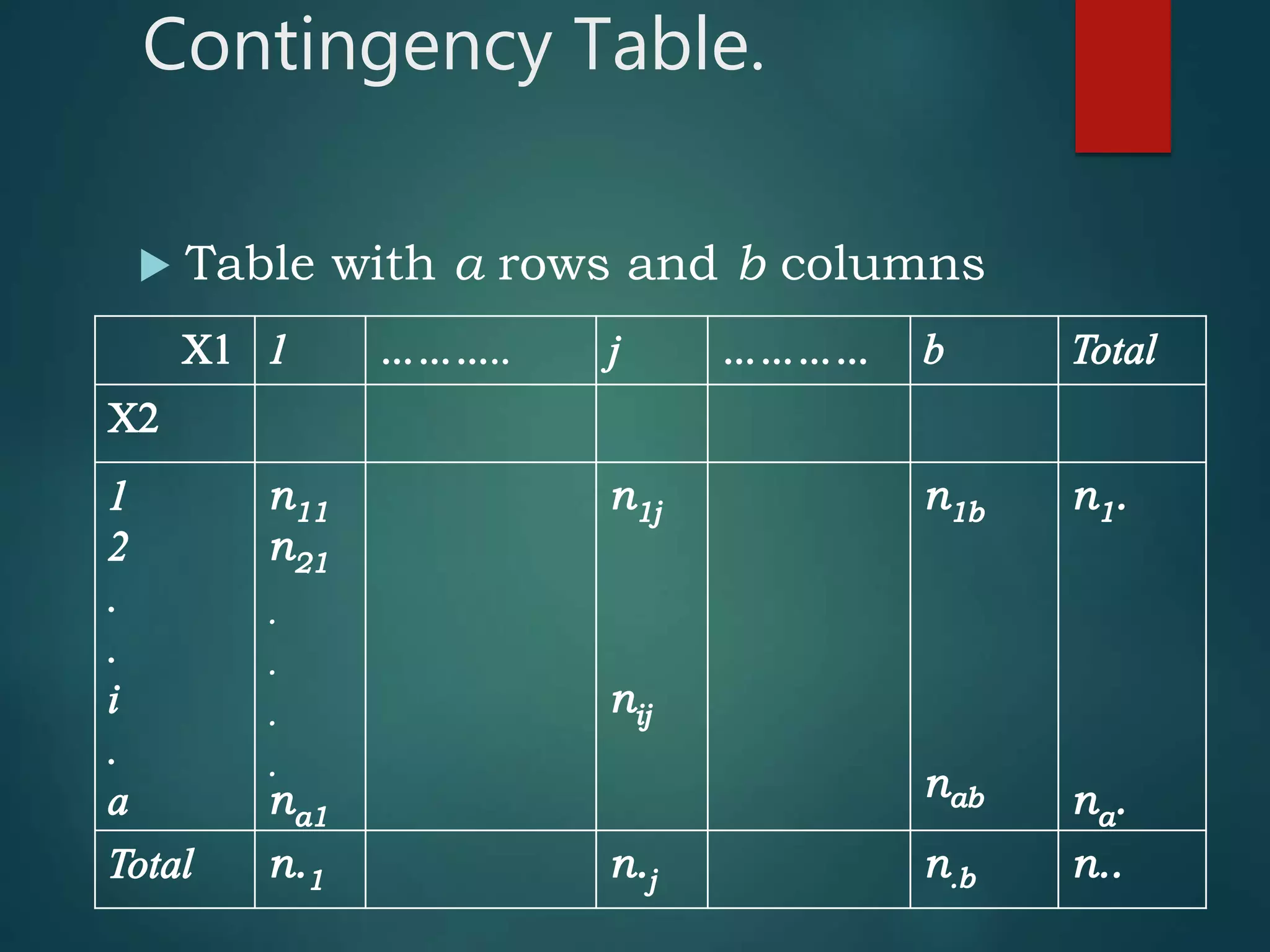
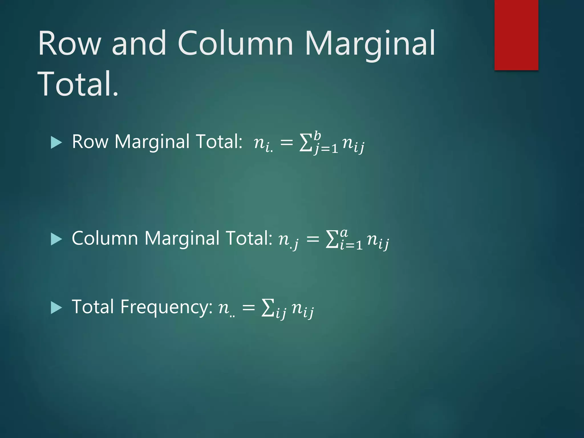
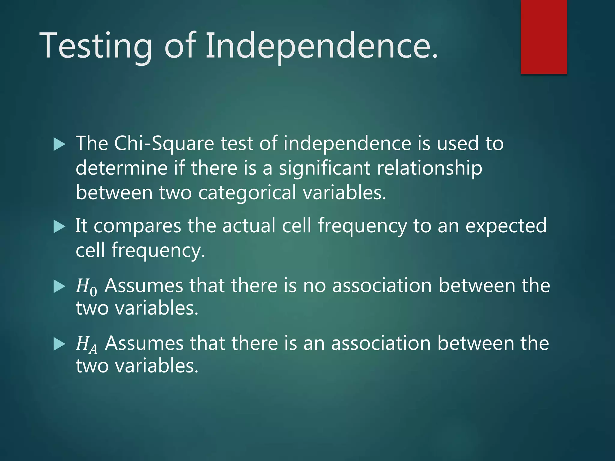
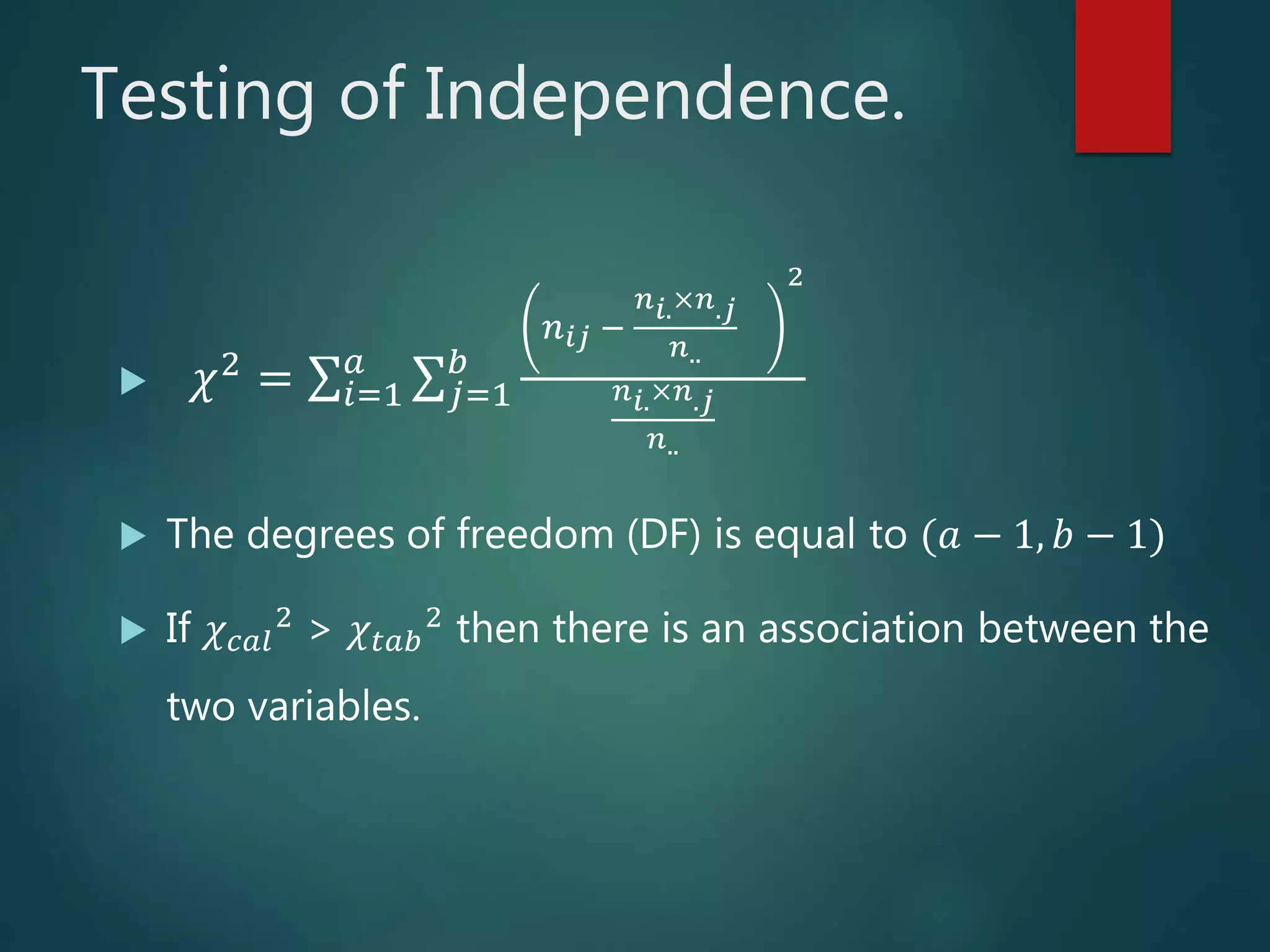
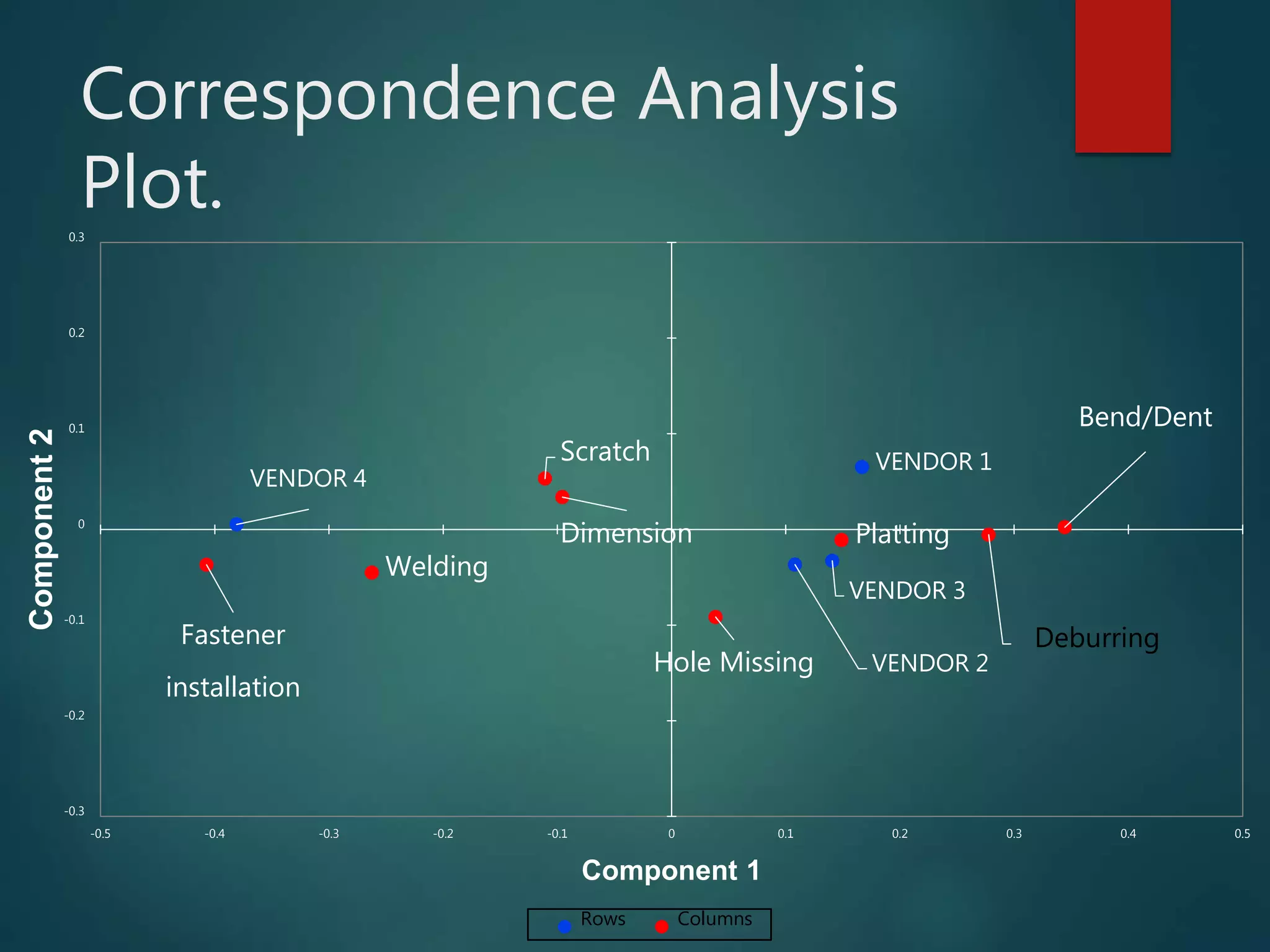
1. Simple
Correspondence
Analysis
Varun G.
Sr. M.Sc (Agril. Stat)
PALB6182

2. Flow of seminar.
1. Introduction.
2. Objectives of Correspondence analysis.
3. Concepts of CA.
4. Advantage and Disadvantage of CA.
5. Case study.
6. Conclusion.
7. References.

3. Correspondance Analysis.
 Correspondence Analysis (CA) is a multivariate
graphical technique designed to explore relationships
among categorical variables.
 Introduced by Benzecri (1973) for uncovering and
understanding the structure and pattern in data in
contingency tables.
 It can be used for both Ordinal and Nominal variables.
 CA is useful in identifying the categories which are
similar.
 CA reduces the Dimensionality.

4. Continue……
 It extends the Factor Analysis in two counts:
1. Handling of categorical variables.
2. Development of perceptual maps of extracted
components.
 CA will show us the relation between rows and
columns.
 It is a compositional method to perceptual mapping
that is based on the categories of a Contengency
table.

5. What is Perceptual Mapping?
 It is a visual representation of a respondent’s
perceptions of objects on two or more dimensions.
 Here each object has a spatial position on the
perceptual map that reflects the similarity or
preference to other objects with regards to the
dimensions of the perceptual map.
 The main objective of the perceptual mapping is to
use the similarities or preferences of the objects in
the multidimensional space.

6. Perceptual Mapping.
 The three basic elements of the perceptual mapping
process are defining the objects, defining the
measure of similarity, and establishing the
dimensions of comparison.
 By this perceptual mapping we can represent the
rows and columns of the contingency table in the
joint space.

7. Objectives of
Correspondence analysis.
 To examine the association among the categories of
just a row or column. The categories can be compared
to see if two can be combined or if they do provide
discrimination.
 Correspondence analysis can be used to know the
association between categories of the rows and
columns.
Eg: Product by age group.

8. Process model for CA
Inputs
• Categorical
variables
• Contingency
table
process
• Compute
measure of
association
• Compute fit
measures
• Create
perceptual
maps
Output
• Perceptual
maps
• Fit measures

9. Contingency Table.
 Contingency tables (also called crosstabs or two-way
tables) are used in statistics to summarize the
relationship between several categorical variables.
 It is a special type of frequency distribution table,
where two variables are shown simultaneously.
 Here the entries are the frequencies of the responses
that fall into each cell of the Matrix.

10. Contingency Table.
 Table with a rows and b columns

11. Row and Column Marginal
Total.
 Row Marginal Total: 𝑛𝑖. = 𝑗=1
𝑏
𝑛𝑖𝑗
 Column Marginal Total: 𝑛.𝑗 = 𝑖=1
𝑎
𝑛𝑖𝑗
 Total Frequency: 𝑛.. = 𝑖𝑗 𝑛𝑖𝑗

12. Testing of Independence.
 The Chi-Square test of independence is used to
determine if there is a significant relationship
between two categorical variables.
 It compares the actual cell frequency to an expected
cell frequency.
 𝐻0 Assumes that there is no association between the
two variables.
 𝐻𝐴 Assumes that there is an association between the
two variables.

13. Testing of Independence.
 𝜒2
= 𝑖=1
𝑎
𝑗=1
𝑏
𝑛 𝑖𝑗 −
𝑛 𝑖.×𝑛.𝑗
𝑛..
2
𝑛 𝑖.×𝑛.𝑗
𝑛..
 The degrees of freedom (DF) is equal to (𝑎 − 1, 𝑏 − 1)
 If 𝜒 𝑐𝑎𝑙
2 > 𝜒𝑡𝑎𝑏
2 then there is an association between the
two variables.

14. Correspondence matrix (P).
 The matrix of relative frequencies is called the
correspondence matrix and is denoted by (P).
 Correspondence matrix is obtained by dividing the
each cell frequency from the total of all the
frequencies.
 It is given by 𝑃 = 𝑝𝑖𝑗 =
𝑛 𝑖𝑗
𝑛..
.

15. Correspondence matrix (P).
X1 1 ……….. j ………… b Total
X2
1
2
.
.
i
.
a
p11
p21
.
.
.
.
pa1
………. p1j
pij
……… p1b
.
.
.
.
pab
p1.
pa.
Total p.1 p.j p.b p..
𝑃 = 𝑝𝑖𝑗 = (𝑛𝑖𝑗/𝑛..)

16. Row and Column vectors.
 Column vector (r) 𝑟 = 𝑃𝑗 = (𝑝1., 𝑝2., … … . . 𝑝 𝑎.)′
Where 𝑗 is an a x 1 vector of 1’s.
 Row vector 𝑐′ = 𝑗′ 𝑃 = (𝑝.1, 𝑝.2, … … . . 𝑝.𝑏)′
Where 𝑗′ is a 1 x b vector of 1’s.
 The elements of vectors r and c are referred as row
and column masses.

17. Row profile (R).
 The row profiles are the row proportions that are
calculated from the counts in the contingency table.
 The value of each cell in the row profiles is the count of
the cell divided by the sum of the counts for the entire
row. The row profile can also be find by the formula
𝑅 = 𝐷𝑟
−1 𝑃
 Where is a diagonal matrix of row vector.
 The row profiles for each row sum to approximately 1
(100%).
𝐷𝑟

18. Row profile (R)
 𝑅 = 𝐷𝑟
−1
𝑃 =
𝑃11
𝑃1.
𝑃12
𝑃1.
⋯
𝑃1𝑏
𝑃1.
𝑃21
𝑃2.
𝑃22
𝑃2.
⋯
𝑃2𝑏
𝑃2.
⋮ ⋮ … ⋮
𝑃 𝑎1
𝑃 𝑎.
𝑃 𝑎2
𝑃 𝑎.
⋯
𝑃 𝑎𝑏
𝑃 𝑎.
 where Diagonal matrix of row vector.
𝐷𝑟=

19. Column profile ( C ).
 The column profiles are the column proportions that are
calculated from the counts in the contingency table.
 The value of each cell in the column profiles table is the
count of the cell divided by the sum of the counts for
the entire column. The column profile can also find by
the formula 𝐶 = 𝑃𝐷𝑐
−1
 Where 𝐷𝑐 is a diagonal matrix of column vector.
 The column profiles for each column sum to
approximately 1 (100%).

20. Column profile (C).
 𝐶 = 𝑃𝐷𝑐
−1
=
𝑃11
𝑃.1
𝑃12
𝑃.2
⋯
𝑃1𝑏
𝑃.𝑎
𝑃21
𝑃.1
𝑃22
𝑃.2
⋯
𝑃2𝑏
𝑃.𝑎
⋮ ⋮ … ⋮
𝑃 𝑎1
𝑃.1
𝑃 𝑎2
𝑃.2
⋯
𝑃 𝑎𝑏
𝑃.𝑎
 𝐷𝑐 Diagonal matrix of column vector

21. Coordinates for Plotting the Row and
Column Profiles.
 Distance matrix (Z)
𝑍 = 𝐷𝑟
−1/2
(𝑃 − 𝑟𝑐′)𝐷𝑐
−1/2
 Where Z is distance matrix, 𝐷𝑟 and 𝐷𝑐 are diagonal
matrices, P is the correspondence matrix, r and c are
row and column masses respectively.
 The matrix Z has rank k = min(a - 1,b - 1).

22. Continue…..
 Single value decomposition
Where,
 Columns of a x k matrix U are eigenvector of 𝑍𝑍′.
 Columns of b x k matrix V are eigenvector of 𝑍′ 𝑍.
 where 𝑑 = 𝑑𝑖𝑎𝑔(𝜆1, 𝜆2,….. 𝜆 𝑘), where 𝜆1
2
, 𝜆2
2
,….., 𝜆 𝑘
2
,
are the nonzero eigenvalues of 𝑍𝑍′
and 𝑍′
𝑍.
𝑍 = 𝑈𝑑𝑉′

23. Continue…..
 The matrix 𝑈 and 𝑉 are orthonormal.
𝑈𝑈′
= 𝐼 = 𝑉′
𝑉
 The values 𝜆1, 𝜆2, … … 𝜆 𝑘 are called singular values
of Z.

24. Row and Column
coordinates.
 Row coordinates (X): 𝑋 = 𝐷𝑟
−1
𝐴d
Where 𝐴 = 𝐷𝑟
1/2
𝑈 and 𝐷𝑟 is a Diagonal matrix of row
masses.
 Column coordinates (Y): 𝑌 = 𝐷𝑐
−1 𝐵𝑑
Where𝐵 = 𝐷𝑐
1/2
𝑉 and 𝐷𝑐 is a Diagonal matrix of
column masses.

25. Continue….
 To plot the coordinates for row profile deviations in two
dimension we plot the rows of the first two columns of X
and to plot the coordinates for column profile deviations in
two dimension, we plot the rows of the first two columns of
Y.
𝑋 =
𝑥11 𝑥12
𝑥21 𝑥22
⋮ ⋮
𝑥 𝑎1 𝑥 𝑎2
𝑌 =
𝑦11 𝑦12
𝑦21 𝑦22
⋮ ⋮
𝑦 𝑏1 𝑦 𝑏2

26. Inertia.
 Inertia measures the variation among the points in the
cross table.
 Total inertia
𝜒2
𝑛
= 𝑖=1
𝑘
𝜆𝑖
2
= 𝑖=1
𝑎
𝑃𝑖. 𝑟𝑖 − 𝑐 ′
𝐷𝑐
−1
(𝑟𝑖 − 𝑐)
 Inertia for 1st dimension is given by 𝜆1
2
𝑖 𝜆𝑖
2
 Inertia for 2nd dimension is given by 𝜆2
2
𝑖 𝜆𝑖
2
 The combined contribution of the two dimensions is given
by
𝜆1
2+𝜆2
2
𝑖=1
𝑘
𝜆 𝑖
2

27. Advantage of CA.
 It can be used with the nominal data rather than
metric ratings of each object on each object. This
capacity enables CA to be used in many situations in
which the more traditional multivariate techniques
are inappropriate.
 CA creates perceptual maps where columns and rows
are simultaneously plotted in the perceptual map
based directly on the association of the variables and
objects.

28. Disadvantage of CA.
 The technique is descriptive/exploratory data analysis
and not at all appropriate for the hypothesis testing.
 There is no method for conclusively determining the
appropriate number of dimensions.
 In CA for the purpose of generalizing, we omit the
objects or attributes which may be critical.
 It is greatly affected by the outliers so we must treat
or exclude them before analysis.

29. Case Study.
 A Framework for Integrated Analysis of Quality
Defects in Supply Chain.
S. Aravindan and J. Maiti,
Indian Institute of Technology Kharagpur, West Bengal,
India.
 The study was carried out between the Vendors and
the Categories of defects of the organization which
manufactures Diagnostic Medical Equipment.

30. Conti...
 The organization has a total of four vendors supplying the
sheet metal components.
 The organization had identified the eight categories of
defects for sheet metal components.
1. Dimension issue.
2. Scratch issue.
3. Plating issue.
4. Bent/Dent issue.
5. Fastener installation problem
6. Welding issue
7. Deburring issue
8. Hole missing issue

31. Contingency table.
BD D DM FI HM P S W
VENDOR 1 150 137 207 91 76 210 185 20
VENDOR 2 142 139 200 120 105 221 185 29
VENDOR 3 146 130 193 114 87 205 148 20
VENDOR 4 57 68 269 260 87 159 239 42
BD - Bend/Dent; D – Deburring; DM – Dimension; FI – Fastener installation; HM – Hole missing
P – Planting issue; S – Scratch; W – Welding;

32. Test for independence.
 Test of independence between the Vendors
and Category of defects:
 Vendors and Category of defect is
dependent.
Chi-square (Observed value) 246.139
Chi-square (Critical value) 32.671
DF 21

33. Row profile.
BD D DM FI HM P S W Sum
VENDOR 1 0.139 0.127 0.192 0.085 0.071 0.195 0.1720.019 1
VENDOR 2 0.124 0.122 0.175 0.105 0.092 0.194 0.1620.025 1
VENDOR 3 0.140 0.125 0.185 0.109 0.083 0.197 0.1420.019 1
VENDOR 4 0.048 0.058 0.228 0.220 0.074 0.135 0.2020.036 1
Mean 0.113 0.108 0.195 0.130 0.080 0.180 0.1700.025 1
BD - Bend/Dent; D – Deburring; DM – Dimension; FI – Fastener installation; HM – Hole missing
P – Planting issue; S – Scratch; W – Welding;

34. Column profile.
BD D DM FI HM P S W Mean
VENDOR 1 0.303 0.289 0.238 0.156 0.214 0.264 0.244 0.180 0.236
VENDOR 2 0.287 0.293 0.230 0.205 0.296 0.278 0.244 0.261 0.262
VENDOR 3 0.295 0.274 0.222 0.195 0.245 0.258 0.196 0.180 0.233
VENDOR 4 0.115 0.143 0.310 0.444 0.245 0.200 0.316 0.378 0.269
Sum 1 1 1 1 1 1 1 1 1
BD - Bend/Dent; D – Deburring; DM – Dimension; FI – Fastener installation; HM – Hole missing
P – Planting issue; S – Scratch; W – Welding;

35. Numerical Summary.
Component 1 Component 2
Name Mass Inertia Coordinates Coordinates
VENDOR 1 0.242 0.140 0.167 0.065
VENDOR 2 0.257 0.068 0.108 -0.037
VENDOR 3 0.235 0.096 0.141 -0.033
VENDOR 4 0.266 0.696 -0.381 0.005
BD 0.111 0.240 0.344 0.002
D 0.107 0.149 0.278 -0.006
DM 0.196 0.038 -0.096 0.034
FI 0.132 0.400 -0.407 -0.037
HM 0.080 0.016 0.039 -0.092
P 0.179 0.072 0.149 -0.011
S 0.170 0.051 -0.111 0.053
W 0.025 0.034 -0.262 -0.045
BD - Bend/Dent; D – Deburring; DM – Dimension; FI – Fastener installation; HM – Hole missing
P – Planting issue; S – Scratch; W – Welding;

36. Eigenvalues and percentages of
inertia:
F1 F2 F3
Eigenvalue 0.053 0.002 0.001
Inertia (%) 95.558 2.950 1.492
Cumulative % 95.558 98.508 100
• The two extracted components explains more than 98%
of total inertia.

37. Scree Plot.

38. Correspondence Analysis
Plot.
VENDOR 1
VENDOR 2
VENDOR 3
VENDOR 4
Bend/Dent
Deburring
Dimension
Fastener
installation
Hole Missing
Platting
Scratch
Welding
-0.3
-0.2
-0.1
0
0.1
0.2
0.3
-0.5 -0.4 -0.3 -0.2 -0.1 0 0.1 0.2 0.3 0.4 0.5
Component2
Component 1
Rows Columns

39. Result.
 Vendor 4 position is far away from other vendor.
 Bend/dent and deburring defects are far away from fastener
installation and welding.
 Vendor 4 has more problem with fastener installation and
welding defects.
 Vendors 1,2 & 3 have relatively more defects related to
bend / dent and deburring.
 The points close to the center of the display have
no/negligible differences.

40. Programs supporting CA.
 SPAD
 SPSS
 SAS
 EDA (Exploratory Data Analysis)
 ViSta from VisualStats
 R software

41. Conclusion
 Correspondence analysis enables the researchers
either to analyze the existing responses or together
responses at the nominal or categorical level.
 It provides not only the relationship between the
rows and columns but also the relationship between
the categories of either row or columns.
 It can provide a joint display of row and column
categories in the same dimensionality.

42. References :
 ARAVINDAN, S. AND J. MAITI., 2012, A framework
for integrated analysis of quality defects in supply
chain. The Quality Management Journal, 19(1): 34-54.
 ERIC, J. B., 2008, Simple Correspondence Analysis of
Nominal-Ordinal Contingency Tables. Journal of Applied
Mathematics and Decision Sciences, 2(9):1-15.
 GREENACRE, M., 2007, Correspondence analysis in
practice. The Quality Management Journal, 5(2): 64-69.

43. Cont……
 HAIR, F. J., ANDERSON, R. E., TATHAM, R. L. AND
BLACK, W. C.,2003, Multivariate data analysis. Journal of
Applied Mathematics and Decision Sciences, 2(1): 582-603.
 HOFFMAN, D. L. AND G. R. FRANKE, 2001,
Correspondence analysis Graphical representation of
categorical data in marketing research. Journal of Marketing
Research,1(5): 213-227.