Download to read offline


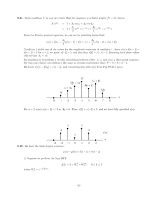
![2.1. We use the graphical approach to compute the convolution:
y[n] = x[n] ∗ h[n]
=
∞
X
k=−∞
x[k]h[n − k]
(a) y[n] = x[n] ∗ h[n]
y[n] = δ[n − 1] ∗ h[n] = h[n − 1]
1 n
2
0 2 3
1
(b) y[n] = x[n] ∗ h[n]
n
2
0 1
-1
5
-2
(c) y[n] = x[n] ∗ h[n]
0 1
2 3 4 5 6 7 8 9 11
10 n
12 13 14 15 16 17 18 19 20
1
2
3
4
5 5
4
3
2 2 2
3
5 5
4
3
2
1
4
(d) y[n] = x[n] ∗ h[n]
n
0 1 2
-1
-2 5
3 4 6
1
3 3
2
1
-1
1
2.2. The response of the system to a delayed step:
y[n] = x[n] ∗ h[n]
=
∞
X
k=−∞
x[k]h[n − k]
=
∞
X
k=−∞
u[k − 4]h[n − k]
2](https://image.slidesharecdn.com/manualsolucoesexextras-210505182102/85/Manual-solucoes-ex_extras-3-320.jpg)
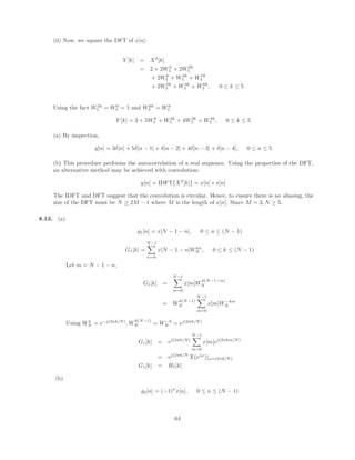
![y[n] =
∞
X
k=4
h[n − k]
Evaluating the above summation:
For n < 4: y[n] = 0
For n = 4: y[n] = h[0] = 1
For n = 5: y[n] = h[1] + h[0] = 2
For n = 6: y[n] = h[2] + h[1] + h[0] = 3
For n = 7: y[n] = h[3] + h[2] + h[1] + h[0] = 4
For n = 8: y[n] = h[4] + h[3] + h[2] + h[1] + h[0] = 2
For n ≥ 9: y[n] = h[5] + h[4] + h[3] + h[2] + h[1] + h[0] = 0
2.3. The output is obtained from the convolution sum:
y[n] = x[n] ∗ h[n]
=
∞
X
k=−∞
x[k]h[n − k]
=
∞
X
k=−∞
x[k]u[n − k]
The convolution may be broken into five regions over the range of n:
y[n] = 0, for n < 0
y[n] =
n
X
k=0
ak
=
1 − a(n+1)
1 − a
, for 0 ≤ n ≤ N1
y[n] =
N1
X
k=0
ak
=
1 − a(N1+1)
1 − a
, for N1 < n < N2
y[n] =
N1
X
k=0
ak
+
n
X
k=N2
a(k−N2)
=
1 − a(N1+1)
1 − a
+
1 − a(n+1)
1 − a
=
2 − a(N1+1)
− a(n+1)
1 − a
, for N2 ≤ n ≤ (N1 + N2)
y[n] =
N1
X
k=0
ak
+
N1+N2
X
k=N2
a(k−N2)
=
N1
X
k=0
ak
+
X
m=0
N1am
3](https://image.slidesharecdn.com/manualsolucoesexextras-210505182102/85/Manual-solucoes-ex_extras-4-320.jpg)
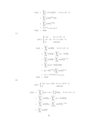
![= 2
N1
X
k=0
ak
= 2 ·
1 − a(N1+1)
1 − a
, for n (N1 + N2)
2.4. Recall that an eigenfunction of a system is an input signal which appears at the output of the system
scaled by a complex constant.
(a) x[n] = 5n
u[n]:
y[n] =
∞
X
k=−∞
h[k]x[n − k]
=
∞
X
k=−∞
h[k]5(n−k)
u[n − k]
= 5n
n
X
k=−∞
h[k]5−k
Becuase the summation depends on n, x[n] is NOT AN EIGENFUNCTION.
(b) x[n] = ej2ωn
:
y[n] =
∞
X
k=−∞
h[k]ej2ω(n−k)
= ej2ωn
∞
X
k=−∞
h[k]e−j2ωk
= ej2ωn
· H(ej2ω
)
YES, EIGENFUNCTION.
(c) ejωn
+ ej2ωn
:
y[n] =
∞
X
k=−∞
h[k]ejω(n−k)
+
∞
X
k=−∞
h[k]ej2ω(n−k)
= ejωn
∞
X
k=−∞
h[k]e−jωk
+ ej2ωn
∞
X
k=−∞
h[k]e−j2ωk
= ejωn
· H(ejω
) + ej2ωn
· H(ej2ω
)
Since the input cannot be extracted from the above expression, the sum of complex exponentials
is NOT AN EIGENFUNCTION. (Although, separately the inputs are eigenfunctions. In general,
complex exponential signals are always eigenfunctions of LTI systems.)
(d) x[n] = 5n
:
y[n] =
∞
X
k=−∞
h[k]5(n−k)
= 5n
∞
X
k=−∞
h[k]5−k
YES, EIGENFUNCTION.
4](https://image.slidesharecdn.com/manualsolucoesexextras-210505182102/85/Manual-solucoes-ex_extras-5-320.jpg)
![(e) x[n] = 5n
ej2ωn
:
y[n] =
∞
X
k=−∞
h[k]5(n−k)
ej2ω(n−k)
= 5n
ej2ωn
∞
X
k=−∞
h[k]5−k
e−j2ωk
YES, EIGENFUNCTION.
2.5. • System A:
x[n] = (
1
2
)n
This input is an eigenfunction of an LTI system. That is, if the system is linear, the output will
be a replica of the input, scaled by a complex constant.
Since y[n] = (1
4 )n
, System A is NOT LTI.
• System B:
x[n] = ejn/8
u[n]
The Fourier transform of x[n] is
X(ejω
) =
∞
X
n=−∞
ejn/8
u[n]e−jωn
=
∞
X
n=0
e−j(ω− 1
8 )n
=
1
1 − e−j(ω− 1
8 )
.
The output is y[n] = 2x[n], thus
Y (ejω
) =
2
1 − e−j(ω− 1
8 )
.
Therefore, the frequency response of the system is
H(ejω
) =
Y (ejω
)
X(ejω)
= 2.
Hence, the system is a linear amplifier. We conclude that System B is LTI, and unique.
• System C: Since x[n] = ejn/8
is an eigenfunction of an LTI system, we would expect the output to
be given by
y[n] = γejn/8
,
where γ is some complex constant, if System C were indeed LTI. The given output, y[n] = 2ejn/8
,
indicates that this is so.
Hence, System C is LTI. However, it is not unique, since the only constraint is that
H(ejω
)|ω=1/8 = 2.
5](https://image.slidesharecdn.com/manualsolucoesexextras-210505182102/85/Manual-solucoes-ex_extras-6-320.jpg)
![2.6. (a) The homogeneous solution yh[n] solves the difference equation when x[n] = 0. It is in the form
yh[n] =
P
A(c)n
, where the c’s solve the quadratic equation
c2
+
1
15
c −
2
5
= 0
So for c = 1/3 and c = −2/5, the general form for the homogeneous solution is:
yh[n] = A1(
1
3
)n
+ A2(−
2
5
)n
(b) We use the z-transform, and use different ROCs to generate the causal and anti-causal impulses
responses:
H(z) =
1
(1 − 1
3 z−1)(1 + 2
5 z−1)
=
5/11
1 − 1
3 z−1
+
6/11
1 + 2
5 z−1
hc[n] =
5
11
(
1
3
)n
u[n] +
6
11
(−
2
5
)n
u[n]
hac[n] = −
5
11
(
1
3
)n
u[−n − 1] −
6
11
(−
2
5
)n
u[−n − 1]
(c) Since hc[n] is causal, and the two exponential bases in hc[n] are both less than 1, it is absolutely
summable. hac[n] grows without bounds as n approaches −∞.
(d)
Y (z) = X(z)H(z)
=
1
1 − 3
5 z−1
·
1
(1 − 1
3 z−1)(1 + 2
5 z−1)
=
−25/44
1 − 1/3z−1
+
55/12
1 + 2/5z−1
+
27/20
1 − 3/5z−1
y[n] =
−25
44
(
1
3
)n
u[n] +
55
12
(−
2
5
)n
u[n] +
27
20
(
3
5
)n
u[n]
2.7. We first re-write the system function H(ejω
):
H(ejω
) = ejπ/4
· e−jω
1 + e−j2ω
+ 4e−j4ω
1 + 1
2 e−j2ω
= ejπ/4
G(ejω
)
Let y1[n] = x[n] ∗ g[n], then
x[n] = cos(
πn
2
) =
ejπn/2
+ e−jπn/2
2
y1[n] =
G(ejπ/2
)ejπn/2
+ G(e−jπ/2
)e−jπn/2
2
Evaluating the frequency response at ω = ±π/2:
G(ej π
2 ) = e−j π
2
1 + e−jπ
+ 4e−j2π
1 + 1
2 e−jπ
= 8e−jπ/2
G(e−j π
2 ) = 8ejπ/2
Therefore,
y1[n] = (8ej(πn/2−π/2)
+ 8ej(−πn/2+π/2)
)/2 = 8 cos(
π
2
n −
π
2
)
and
y[n] = ejπ/4
y1[n] = 8ejπ/4
cos(
π
2
n −
π
2
)
6](https://image.slidesharecdn.com/manualsolucoesexextras-210505182102/85/Manual-solucoes-ex_extras-7-320.jpg)
![2.8. (a) Notice that
x[n] = x0[n − 2] + 2x0[n − 4] + x0[n − 6]
Since the system is LTI,
y[n] = y0[n − 2] + 2y0[n − 4] + y0[n − 6],
and we get sequence shown here:
1
-1
7 8
6
5
4
3
2
1
0
-2
2
(b) Since
y0[n] = −1x0[n + 1] + x0[n − 1] = x0[n] ∗ (−δ[n + 1] + δ[n − 1]),
h[n] = −δ[n + 1] + δ[n − 1]
2.9. For (−1 a 0), we have
X(ejω
) =
1
1 − ae−jω
(a) real part of X(ejω
):
XR(ejω
) =
1
2
· [X(ejω
) + X∗
(ejω
)]
=
1 − a cos(ω)
1 − 2a cos(ω) + a2
(b) imaginary part:
XI(ejω
) =
1
2j
· [X(ejω
) − X∗
(ejω
)]
=
−a sin(ω)
1 − 2a cos(ω) + a2
(c) magnitude:
|X(ejω
)| = [X(ejω
)X∗
(ejω
)]
1
2
=
1
1 − 2acos(ω) + a2
1
2
(d) phase:
6 X(ejω
) = arctan
−a sin(ω)
1 − a cos(ω)
2.10. x[n] can be rewritten as:
x[n] = cos(
5πn
2
)
= cos(
πn
2
)
=
ej πn
2
2
+
e−j πn
2
2
.
7](https://image.slidesharecdn.com/manualsolucoesexextras-210505182102/85/Manual-solucoes-ex_extras-8-320.jpg)
![We now use the fact that complex exponentials are eigenfunctions of LTI systems, we get:
y[n] = e−j π
8
ej πn
2
2
+ ej π
8
e−j πn
2
2
=
ej( πn
2 − π
8 )
2
+
e−j( πn
2 − π
8 )
2
= cos(
π
2
(n −
1
4
)).
2.11. First x[n] goes through a lowpass filter with cutoff frequency 0.5π. Since the cosine has a frequency of
0.6π, it will be filtered out. The delayed impulse will be filtered to a delayed sinc and the constant will
remain unchanged. We thus get:
w[n] = 3
sin(0.5π(n − 5))
π(n − 5)
+ 2.
y[n] is then given by:
y[n] = 3
sin(0.5π(n − 5))
π(n − 5)
− 3
sin(0.5π(n − 6))
π(n − 6)
.
2.12. Since system 1 is memoryless, it is time invariant. The input, x[n] is periodic in ω, therefore w[n] will
also be periodic in ω. As a consequence, y[n] is periodic in ω and so is A.
8](https://image.slidesharecdn.com/manualsolucoesexextras-210505182102/85/Manual-solucoes-ex_extras-9-320.jpg)

![3.1. (a)
H(z) =
1 − 1
2 z−2
(1 − 1
2 z−1)(1 − 1
4 z−1)
= −4 +
5 + 7
2 z−1
1 − 3
4 z−1 + 1
8 z−2
= −4 −
2
1 − 1
2 z−1
+
7
1 − 1
4 z−1
h[n] = −4δ[n] − 2
1
2
n
u[n] + 7
1
4
n
u[n]
(b)
y[n] −
3
4
y[n − 1] +
1
8
y[n − 2] = x[n] −
1
2
x[n − 2]
3.2.
H(z) =
3 − 7z−1
+ 5z−2
1 − 5
2 z−1 + z−2
= 5 +
1
1 − 2z−1
−
3
1 − 1
2 z−1
h[n] stable ⇒ h[n] = 5δ[n] − 2n
u[−n − 1] − 3
1
2
n
u[n]
(a)
y[n] = h[n] ∗ x[n] =
n
X
k=−∞
h[k]
=
−
n
X
k=−∞
2k
= −2n+1
n 0
−
−1
X
k−∞
2k
+ 5 −
n
X
k=0
3
1
2
k
= 4 − 3
1 − (1
2 )n+1
1 − 1
2
= −2 + 3
1
2
n
n ≥ 0
= −2u[n] + 3
1
2
n
u[n] − 2n+1
u[−n − 1]
(b)
Y (z) =
1
1 − z−1
H(z) = −2
1
1 − z−1
+ 2
1
1 − 2z−1
+ 3
1
1 − 1
2 z−1
,
1
2
|z| 2
y[n] = −2u[n] − 2(2)n
u[−n − 1] + 3
1
2
n
u[n]
3.3.
Y (z) =
z−1
+ z−2
(1 − 1
2 z−1)(1 + 1
3 z−1)
·
2
1 − z−1
|z| 1
Therefore using a contour C that lies outside of |z| = 1 we get
y[1] =
1
2πj
I
C
2(z + 1)zn
dz
(z − 1
2 )(z + 1
3 )(z − 1)
=
2(1
2 + 1)(1
2 )
(1
2 + 1
3 )(1
2 − 1)
+
2(−1
3 + 1)(−1
3 )
(−1
3 − 1
2 )(−1
3 − 1)
+
2(1 + 1)(1)
(1 − 1
2 )(1 + 1
3 )
= −
18
5
−
2
5
+ 6 = 2
10](https://image.slidesharecdn.com/manualsolucoesexextras-210505182102/85/Manual-solucoes-ex_extras-11-320.jpg)
![3.4. (a)
X(z) =
z10
(z − 1
2 )(z − 3
2 )10(z + 3
2 )2(z + 5
2 )(z + 7
2 )
Stable ⇒ ROC includes |z| = 1. Therefore, the ROC is 1
2 |z| 3
2 .
(b) x[−8] = Σ[residues of X(z)z−9
inside C], where C is contour in ROC (say the unit circle).
x[8] = Σ
residues of
z
(z − 1
2 )(z − 3
2 )10(z + 3
2 )2(z + 5
2 )(z + 7
2 )
inside unit circle
First order pole at z = 1
2 is only one inside the unit circle. Therefore
x[−8] =
1
2
(1
2 − 3
2 )10(1
2 + 3
2 )2(1
2 + 5
2 )(1
2 + 7
2 )
=
1
96
3.5. (a)
X(z) =
−1
3
1 − 1
2 z−1
+
4
3
1 − 2z−1
The ROC is 1
2 |z| 2.
(b) The following figure shows the pole-zero plot of Y (z). Since X(z) has poles at 0.5 and 2, the poles
at 1 and -0.5 are due to H(z). Since H(z) is causal, its ROC is |z| 1. The ROC of Y (z) must
contain the intersection of the ROC of X(z) and the ROC of H(z). Hence the ROC of Y (z) is
1 |z| 2.
−1 −0.5 0 0.5 1 1.5 2
−1.5
−1
−0.5
0
0.5
1
1.5
Real part
Imaginary
part
Pole−zero plot of Y(z)
−1 1
−0.5 2
(c)
H(z) =
Y (z)
X(z)
=
1+z−1
(1−z−1)(1+ 1
2 z−1)(1−2z−1)
1
(1−12z−1)(1−2z−1)
=
(1 + z−1
)(1 − 1
2 z−1
)
(1 − z−1)(1 − 1
2 z−1)
= 1 +
2
3
1 − z−1
+
−2
3
1 + 1
2 z−1
Taking the inverse z-transform, we find
h[n] = δ[n] +
2
3
u[n] −
2
3
(−
1
2
)n
u[n]
(d) Since H(z) has a pole on the unit circle, the system is not stable.
11](https://image.slidesharecdn.com/manualsolucoesexextras-210505182102/85/Manual-solucoes-ex_extras-12-320.jpg)

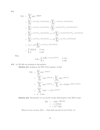
![4.1. (a) Keeping in mind that after sampling, ω = ΩT , the Fourier transform of x[n] is
Ω1
Ω2
X ( j Ω)
c
−π π
π ω
jω
Ω Ω
1 2 Ω
X (e )
(b) A straight-forward application of the Nyquist criterion would lead to an incorrect conclusion that
the sampling rate is at least twice the maximum frequency of xc(t), or 2Ω2. However, since the
spectrum is bandpass, we only need to ensure that the replications in frequency which occur as a
result of sampling do not overlap with the original. (See the following figure of Xs(jΩ).) Therefore,
we only need to ensure
Ω2 −
2π
T
Ω1 =⇒ T
2π
∆Ω
Ω2
Ω1
Ω2
− 2π
Τ
Ω
)
Ω
X (j
s
(c) The block diagram along with the frequency response of h(t) is shown here:
Ω Ω Ω
1 2
convert
sequence
to impulse
train
bandpass
h(t)
filter
x[n] x(t)
4.2. (a)
ω = ΩT, T =
2π
Ω0
−π π ω
1/Τ
X(e )
ω
j
13](https://image.slidesharecdn.com/manualsolucoesexextras-210505182102/85/Manual-solucoes-ex_extras-14-320.jpg)
![(b) To recover simply filter out the undesired parts of X(ejω
).
Bandpass
Filter
x[n] c
x (t)
Ω
−π π
−2π 2π
/T /T /T /T
T
(c)
T ≤
2π
Ω0
4.3. First we show that Xs(ejω
) is just a sum of shifted versions of X(ejω
):
xs[n] =
x[n], n = Mk, k = 0, ±1, ±2
0, otherwise
=
1
M
M−1
X
k=0
ej(2πkn/M)
!
x[n]
Xs(ejω
) =
∞
X
n=−∞
xs[n]e−jωn
=
∞
X
n=−∞
1
M
M−1
X
k=0
x[n]ej(2πkn/M)
e−jωn
=
1
M
M−1
X
k=0
∞
X
n=−∞
x[n]e−j[ω−(2πk/M)]n
=
1
M
M−1
X
k=0
X
ej[ω−(2πk/M)]
Additionally, Xd(ejω
) is simply Xs(ejω
) with the frequency axis expanded by a factor of M:
Xd(ejω
) =
∞
X
n=−∞
Xs[Mn]e−jωn
=
∞
X
l=−∞
xs[l]e−j(ω/M)l
= Xs
ej(ω/M)
(a) (i) Xs(ejω
) and Xd(ejω
) are sketched below for M = 3, ωH = π/2.
14](https://image.slidesharecdn.com/manualsolucoesexextras-210505182102/85/Manual-solucoes-ex_extras-15-320.jpg)
![1/3
s
−2π/3
−π/2 2π/3
π/2
ω
j
ω
−π π
X (e )
1/3
ω
j
ω
d
−π π 2π
−2π
X (e )
(ii) Xs(ejω
) and Xd(ejω
) are sketched below for M = 3, ωH = π/4.
1/3
ω
j
ω
d
−π π 2π
−2π
X (e )
1/3
s
−2π/3 2π/3
ω
j
ω
−π π
X (e )
−π/4 π/4
(b) From the definition of Xs(ejω
), we see that there will be no aliasing if the signal is bandlimited to
π/M. In this problem, M = 3. Thus the maximum value of ωH is π/3.
4.4. Parseval’s Theorem: ∞
X
n=−∞
|x[n]|2
=
1
2π
Z π
−π
|X(ejω
)|2
dω
When we upsample, the added samples are zeros, so the upsampled signal xu[n] has the same energy as
the original x[n]:
∞
X
n=−∞
|x[n]|2
=
∞
X
n=−∞
|xu[n]|2
,
and by Parseval’s theorem:
1
2π
Z π
−π
|X(ejω
)|2
dω =
1
2π
Z π
−π
|Xu(ejω
)|2
dω.
Hence the amplitude of the Fourier transform does not change.
When we downsample, the downsampled signal xd[n] has less energy than the original x[n] because some
samples are discarded. Hence the amplitude of the Fourier transform will change after downsampling.
15](https://image.slidesharecdn.com/manualsolucoesexextras-210505182102/85/Manual-solucoes-ex_extras-16-320.jpg)
![4.5. (a) Yes, the system is linear because each of the subblocks is linear. The C/D step is defined by
x[n] = xc(nT ), which is clearly linear. The DT system is an LTI system. The D/C step consists
of converting the sequence to impulses and of CT LTI filtering, both of which are linear.
(b) No, the system is not time-invariant.
For example, suppose that h[n] = δ[n], T = 5 and xc(t) = 1 for −1 ≤ t ≤ 1. Such a system would
result in x[n] = δ[n] and yc(t) = sinc(π/5). Now suppose we delay the input to be xc(t − 2). Now
x[n] = 0 and yc(t) = 0.
4.6. We can analyze the system in the frequency domain:
jω
jω
1
H (e )
jω
1
2
Y (e )
jω
X(e ) 1
2jω H (e )
X(e )
2
2jω
X(e )
Y1(ejω
) is X(e2jω
)H1(ejω
) downsampled by 2:
Y1(ejω
) =
1
2
n
X(e2jω/2
)H1(ejω/2
) + X(e(2j(ω−2π)/2
)H1(ej(ω−2π)/2
)
o
=
1
2
n
X(ejω
)H1(ejω/2
) + X(ej(ω−2π)
)H1(ej( ω
2 −π)
)
o
=
1
2
n
H1(ejω/2
) + H1(ej( ω
2 −π)
)
o
X(ejω
)
= H2(ejω
)X(ejω
)
H2(ejω
) =
1
2
n
H1(ejω/2
) + H1(ej( ω
2 −π)
)
o
4.7.
Xc(jΩ) = 0 |Ω| ≥ 4000π
Y (jΩ) = |Ω|Xc(jΩ), 1000π ≤ |Ω| ≤ 2000π
Since only half the frequency band of Xc(jΩ) is needed, we can alias everything past Ω = 2000π. Hence,
T = 1/3000 s.
Now that T is set, figure out H(ejω
) band edges.
ω1 = Ω1T ⇒ ω1 = 2π · 500 · 1
3000 ⇒ ω1 =
π
3
ω2 = Ω2T ⇒ ω2 = 2π · 1000 · 1
3000 ⇒ ω2 =
2π
3
H(ejω
) =
|ω| π
3 ≤ |ω| ≤ 2π
3
0 0 ≤ |ω| π
3 , 2π
3 |ω| ≤ π
4.8.
Xc(jΩ) = 0, |Ω|
π
T
yr(t) =
Z t
−∞
xc(τ)dτ =⇒ Hc(jΩ) =
1
jΩ
In discrete-time, we want
H(ejω
) =
1
jω , −π ≤ ω ≤ π
0, otherwise
16](https://image.slidesharecdn.com/manualsolucoesexextras-210505182102/85/Manual-solucoes-ex_extras-17-320.jpg)
![|H(e )|
jω
ω
π 2π
−π
−2π
−π
ω
π
−π 2π
−2π
jω
arg(H(e ))
4.9. (a) The highest frequency is π/T = π × 10000.
(b)
−1 −0.8 −0.6 −0.4 −0.2 0 0.2 0.4 0.6 0.8 1
−100
−50
0
50
100
Normalized frequency (Nyquist == 1)
Phase
(degrees)
−1 −0.8 −0.6 −0.4 −0.2 0 0.2 0.4 0.6 0.8 1
−60
−50
−40
−30
−20
−10
0
10
Normalized frequency (Nyquist == 1)
Magnitude
Response
(dB)
(c) To filter the 60Hz out,
ω0 = T Ω =
1
10, 000
· 2π · 60 =
3π
250
4.10. (a) Since there is no aliasing involved in this process, we may choose T to be any value. Choose T = 1
for simplicity. Xc(jΩ) = 0, |Ω| ≥ π/T . Since Yc(jΩ) = Hc(jΩ)Xc(jΩ), Yc(jΩ) = 0, |Ω| ≥ π/T .
Therefore, there will be no aliasing problems in going from yc(t) to y[n].
Recall the relationship ω = ΩT . We can simply use this in our system conversion:
H(ejω
) = e−jω/2
H(jΩ) = e−jΩT/2
= e−jΩ/2
, T = 1
Note that the choice of T and therefore H(jΩ) is not unique.
(b)
cos
5π
2
n −
π
4
=
1
2
h
ej( 5π
2 n− π
4 )
+ e−j( 5π
2 n− π
4 )
i
=
1
2
e−j(π/4)
ej(5π/2)n
+
1
2
ej(π/4)
e−j(5π/2)n
17](https://image.slidesharecdn.com/manualsolucoesexextras-210505182102/85/Manual-solucoes-ex_extras-18-320.jpg)
![Since H(ejω
) is an LTI system, we can find the response to each of the two eigenfunctions separately.
y[n] =
1
2
e−j(π/4)
H
ej(5π/2)
ej(5π/2)n
+
1
2
ej(π/4)
H
e−j(5π/2)
e−j(5π/2)n
Since H(ejω
) is defined for 0 ≤ |ω| ≤ π we must evaluate the frequency at the baseband, i.e.,
5π/2 ⇒ 5π/2 − 2π = π/2. Therefore,
y[n] =
1
2
e−j(π/4)
H
ej(5π/2)
ej(5π/2)n
+
1
2
ej(π/4)
H
e−j(5π/2)
e−j(5π/2)n
=
1
2
ej[(5π/2)n−(π/2)]
+ e−j[(5π/2)n−(π/2)]
= cos
5π
2
n −
π
2
n
0
-1
1
y[n]
4.11. The frequency response H(ejω
) = Hc(jΩ/T ). Finding that
Hc(jΩ) =
1
(jΩ)2 + 4(jΩ) + 3
,
H(ejω
) =
1
(10jω)2 + 4(10jω) + 3
=
1
−100ω2 + 3 + 40jω
4.12. (a) Since ΩT = ω, (2π · 100)T = π
2 ⇒ T = 1
400
(b) The downsampler has M = 2. Since x[n] is bandlimited to π
M , there will be no aliasing. The
frequency axis simply expands by a factor of 2.
For yc(t) = xc(t) ⇔ Yc(jΩ) = Xc(jΩ).
Therefore ΩT 0
⇒ 2π · 100T 0
⇒ T 0
= 1
200 .
4.13. In both systems, the speech was filtered first so that the subsequent sampling results in no aliasing.
Therefore, going s[n] to s1[n] basically requires changing the sampling rate by a factor of 3kHz/5kHz =
3/5. This is done with the following system:
Digital LPF
gain = 3
cutoff =π/3
3 5
1
s[n] s [n]
4.14. Xc(jΩ) is drawn below.
X (j )
Ω
Ω
c
1/T
18](https://image.slidesharecdn.com/manualsolucoesexextras-210505182102/85/Manual-solucoes-ex_extras-19-320.jpg)
![xc(t) is sampled at sampling period T , so there is no aliasing in x[n].
X(e )
jω
ω
π
−π
1/T
Inserting L − 1 zeros between samples compresses the frequency axis.
V(e )
jω
ω
π/
L
−π/ L
1/LT
The filter H(ejω
) removes frequency components between π/L and π.
j
ω
W(e )
−π/ L π/L
1/LT
ω
The multiplication by (−1)n
shifts the center of the frequency band from 0 to π.
Y(e )
jω
ω
−π π
1/LT
The D/C conversion maps the range −π to π to the range −π/T to π/T .
Y (j )
c
Ω
Ω
π L/T
−π L/T
1/L
4.15. (a)
h[n] = 0, |n| (RL − 1)
Therefore, for causal system delay by RL − 1 samples.
(b) General interpolator condition:
h[0] = 1
h[kL] = 0, k = ±1, ±2, . . .
(c)
y[n] =
(RL−1)
X
k=−(RL−1)
h[k]v[n − k] = h[0]v[n] +
RL−1
X
k=1
h[n](v[n − k] + v[n + k])
This requires only RL-1 multiplies, (assuming h[0] = 1.)
19](https://image.slidesharecdn.com/manualsolucoesexextras-210505182102/85/Manual-solucoes-ex_extras-20-320.jpg)
![(d)
y[n] =
n+(RL−1)
X
k=n−(RL−1)
v[k]h[n − k]
If n = mL (m an integer), then we don’t have any multiplications since h[0] = 1 and the other
non-zero samples of v[k] hit at the zeros h[n]. Otherwise the impulse response spans 2RL − 1
samples of v[n], but only 2R of these are non-zero. Therefore, there are 2R multiplies.
4.16. (a) See figures below.
(b) From part(a), we see that
Yc(jΩ) = Xc(j(Ω −
2π
T
)) + Xc(j(Ω +
2π
T
))
Therefore,
yc(t) = 2xc(t) cos(
2π
T
t)
X(e )
jω
π
−π ω
1/T
X (e )
jω
e
π/4 3π/4 5π/4
−π/4
−3π/4
−5π/4 ω
1/T
π/4 3π/4
−π/4
−3π/4 ω
e
jω
4/T
Y (e )
Y (j Ω)
c
−3π/Τ π/Τ 3π/Τ
−π/Τ
1
Ω
4.17. (a) The Nyquist criterion states that xc(t) can be recovered as long as
2π
T
≥ 2 × 2π(250) =⇒ T ≤
1
500
.
In this case, T = 1/500, so the Nyquist criterion is satisfied, and xc(t) can be recovered.
(b) Yes. A delay in time does not change the bandwidth of the signal. Hence, yc(t) has the same
bandwidth and same Nyquist sampling rate as xc(t).
20](https://image.slidesharecdn.com/manualsolucoesexextras-210505182102/85/Manual-solucoes-ex_extras-21-320.jpg)
![(c) Consider first the following expressions for X(ejω
) and Y (ejω
):
X(ejω
) =
1
T
Xc(jΩ) |Ω= ω
T
=
1
500
Xc(j500ω)
Y (ejω
) =
1
T
Yc(jΩ) |Ω= ω
T
=
1
T
e−jΩ/1000
Xc(jΩ) |Ω= ω
T
=
1
500
e−jω/2
Xc(j500ω)
= e−jω/2
X(ejω
)
Hence, we let
H(ejω
) =
2e−jω
, |ω| π
2
0, otherwise
Then, in the following figure,
R(ejω
) = X(ej2ω
)
W(ejω
) =
2e−jω
X(ej2ω
), |ω| π
2
0, otherwise
Y (ejω
) = e−jω/2
X(ejω
)
x[n] r[n] w[n] y[n]
2 2
H
(d) Yes, from our analysis above,
H2(ejω
) = e−jω/2
4.18. (a) Notice first that
Xc(jΩ) =
Fc(jΩ)|Haa(jΩ)|e−jΩ3
, |Ω| ≤ 400π
Ec(jΩ)|Haa(jΩ)|e−jΩ3
, 400π ≤ |Ω| ≤ 800π
0, otherwise
For the given T = 1/800, there is no aliasing from the C/D conversion. Hence, the equivalent CT
transfer function Hc(jΩ) can be written as
Hc(jΩ) =
H(ejω
)|ω=ΩT , |Ω| ≤ π/T
0, otherwise
Furthermore, since Yc(jΩ) = Hc(jΩ)Xc(jΩ), the desired tranfer function is
Hc(jΩ) =
ejΩ3
, |Ω| ≤ 400π
0, otherwise
Combining the two previous equations, we find
H(ejω
) =
ej(800ω)3
, |ω| ≤ π/2
0, π/2 ≤ |ω| ≤ π
(b) Some aliasing will occur if 2π/T 1600π. However, this is fine as long as the aliasing affects only
Ec(jΩ) and not Fc(jΩ), as we show below:
21](https://image.slidesharecdn.com/manualsolucoesexextras-210505182102/85/Manual-solucoes-ex_extras-22-320.jpg)

![4.20. Notice first that since xc(t) is time-limited,
A =
Z 10
0
xc(t)dt =
Z ∞
−∞
xc(t)dt = Xc(jΩ)|Ω=0.
To estimate Xc(j · 0) by DT processing, we need to sample only fast enough so that Xc(j · 0) is not
aliased. Hence, we pick
2π/T = 2π × 104
=⇒ T = 10−4
.
The resulting spectrum satisfies
X(ej·0
) =
1
T
Xc(j · 0)
Further,
X(ej·0
) =
∞
X
n=−∞
x[n].
Therefore, we pick h[n] = T u[n], which makes the system an accumulator. Our estimate  is the output
y[n] at n = 10/(10−4
) = 105
, when all of the non-zero samples of x[n] have been added-up. This is
an exact estimate given our assumption of both band- and time-limitedness. Since the assumption can
never be exactly satisfied, however, this method only gives an approximate estimate for actual signals.
The overall system is as follows:
C/D
x (t)
c
T = 1/10000
h[n] = T u[n]
y[n] A = y[100000]
4.21. (a) Notice that
y0[n] = x[3n]
y1[n] = x[3n + 1]
y2[n] = x[3n + 2],
and therefore,
x[n] =
y0[n/3], n = 3k
y1[(n − 1)/3], n = 3k + 1
y2[(n − 2)/3], n = 3k + 2
(b) Yes. Since the bandwidth of the filters are 2π/3, there is no aliasing introduced by downsampling.
Hence to reconstruct x[n], we need the system shown in the following figure:
3
3
H (z)
H (z)
0
1
2
y [n]
y [n]
y [n]
0
1
2
x[n]
H (z)
3
3
3
3
(c) Yes, x[n] can be reconstructed from y3[n] and y4[n] as demonstrated by the following figure:
23](https://image.slidesharecdn.com/manualsolucoesexextras-210505182102/85/Manual-solucoes-ex_extras-24-320.jpg)
![y [n]
w [n]
w [n] y [n] v [n]
v [n] x[n]
s[n]
2
2
2
2
3
4
3
4
3
4
x[n]
3
4 4
H (z)
H (z)
H (z)
In the following discussion, let xe[n] denote the even samples of x[n], and xo[n] denote the odd
samples of x[n]:
xe[n] =
x[n], n even
0, n odd
xo[n] =
0, n even
x[n], n odd
In the figure, y3[n] = x[2n], and hence,
v3[n] =
x[n], n even
0, n odd
= xe[n]
Furthermore, it can be verified using the IDFT that the impulse response h4[n] corresponding to
H4(ejω
) is
h4[n] =
−2/(jπn), n odd
0, otherwise
Notice in particular that every other sample of the impulse response h4[n] is zero. Also, from the
form of H4(ejω
), it is clear that H4(ejω
)H4(ejω
) = 1, and hence h4[n] ∗ h4[n] = δ[n].
Therefore,
v4[n] =
y4[n/2], n even
0, n odd
=
w4[n], n even
0, n odd
=
(x ∗ h4)[n], n even
0, n odd
= xo[n] ∗ h4[n]
where the last equality follows from the fact that h4[n] is non-zero only in the odd samples.
Now, s[n] = v4[n]∗h4[n] = xo[n]∗h4[n]∗h4[n] = xo[n], and since x[n] = xe[n]+xo[n], s[n]+v3[n] =
x[n].
24](https://image.slidesharecdn.com/manualsolucoesexextras-210505182102/85/Manual-solucoes-ex_extras-25-320.jpg)

![5.1.
H(z) =
1 − a−1
z−1
1 − az−1
=
Y (z)
X(z)
, causal, so ROC is |z| a
(a) Cross multiplying and taking the inverse transform
y[n] − ay[n − 1] = x[n] −
1
a
x[n − 1]
(b) Since H(z) is causal, we know that the ROC is |z| a. For stability, the ROC must include the
unit circle. So, H(z) is stable for |a| 1.
(c) a = 1
2
Re
Im |z| 1/2
1/2 2
(d)
H(z) =
1
1 − az−1
−
a−1
z−1
1 − az−1
, |z| a
h[n] = (a)n
u[n] −
1
a
(a)n−1
u[n − 1]
(e)
H(ejω
) = H(z)|z=ejω =
1 − a−1
e−jω
1 − ae−jω
|H(ejω
)|2
= H(ejω
)H∗
(ejω
) =
1 − a−1
e−jω
1 − ae−jω
·
1 − a−1
ejω
1 − aejω
|H(ejω
)| =
1 + 1
a2 − 2
a cos ω
1 + a2 − 2a cosω
1
2
=
1
a
a2
+ 1 − 2a cosω
1 + a2 − 2a cosω
1
2
=
1
a
5.2. (a) Type I:
A(ω) =
M/2
X
n=0
a[n] cos ωn
cos 0 = 1, cos π = −1, so there are no
restrictions.
26](https://image.slidesharecdn.com/manualsolucoesexextras-210505182102/85/Manual-solucoes-ex_extras-27-320.jpg)
![Type II:
A(ω) =
(M+1)/2
X
n=1
b[n] cosω
n −
1
2
cos 0 = 1, cos nπ − π
2
= 0. So H(ejπ
) = 0.
Type III:
A(ω) =
M/2
X
n=0
c[n] sin ωn
sin 0 = 0, sin nπ = 0, so H(ej0
) = H(ejπ
) = 0.
Type IV:
A(ω) =
(M+1)/2
X
n=1
d[n] sin ω
n −
1
2
sin 0 = 0, sin nπ − π
2
6= 0, so just H(ej0
) = 0.
(b) Type I Type II Type III Type IV
Lowpass Y Y N N
Bandpass Y Y Y Y
Highpass Y N N Y
Bandstop Y N N N
Differentiator Y N N Y
5.3. (a) Taking the z-transform of both sides and rearranging
H(z) =
Y (z)
X(z)
=
−1
4 + z−2
1 − 1
4 z−2
Since the poles and zeros {2 poles at z = ±1/2, 2 zeros at z = ±2} occur in conjugate reciprocal
pairs the system is allpass. This property is easy to recognize since, as in the system above,
the coefficients of the numerator and denominator z-polynomials get reversed (and in general
conjugated).
(b) It is a property of allpass systems that the output energy is equal to the input energy. Here is the
proof.
27](https://image.slidesharecdn.com/manualsolucoesexextras-210505182102/85/Manual-solucoes-ex_extras-28-320.jpg)
![N−1
X
n=0
|y[n]|2
=
∞
X
n=−∞
|y[n]|2
=
1
2π
Z π
−π](https://image.slidesharecdn.com/manualsolucoesexextras-210505182102/85/Manual-solucoes-ex_extras-29-320.jpg)


![2
= 1 since h[n] is allpass)
=
∞
X
n=−∞
|x[n]|2
(by Parseval’s theorem)
=
N−1
X
n=0
|x[n]|2
= 5
5.4. The statement is false. A non-causal system can indeed have a positive constant group delay.
For example, consider the non-causal system
h[n] = δ[n + 1] + δ[n] + 4δ[n − 1] + δ[n − 2] + δ[n − 3]
This system has the frequency response
H(ejω
) = ejω
+ 1 + 4e−jω
+ e−j2ω
+ e−j3ω
= e−jω
(ej2ω
+ ejω
+ 4 + e−jω
+ e−j2ω
)
= e−jω
(4 + 2 cos(ω) + 2 cos(2ω))](https://image.slidesharecdn.com/manualsolucoesexextras-210505182102/85/Manual-solucoes-ex_extras-45-320.jpg)


![= 4 + 2 cos(ω) + 2 cos(2ω)
6 H(ejω
) = −ω
grd[H(ejω
)] = 1
5.5. Making use of some DTFT properties can aide in the solution of this
problem. First, note that
h2[n] = (−1)n
h1[n]
h2[n] = e−jπn
h1[n]
Using the DTFT property that states that modulation in the time domain corresponds to a shift in the
frequency domain,
H2(ejω
) = H1(ej(ω+π)
)
Consequently, H2(ejω
) is simply H1(ejω
) shifted by π. The ideal low pass filter has now become the
ideal high pass filter, as shown below.
28](https://image.slidesharecdn.com/manualsolucoesexextras-210505182102/85/Manual-solucoes-ex_extras-49-320.jpg)
![ω
−π −π/2 0 π/2 π
1
H
1
(e
jω
)
ω
−π −π/2 0 π/2 π
1
H
2
(e
jω
)
5.6. (a)
H(z) =
(z + 1
2 )(z − 1
2 )
zM
= z−(M−2)
1 −
1
4
z−2
n
M−2 M−1
M
1
−1/4
(b)
w[n] = x[n − (M − 2)] −
1
4
x[n − M]
y[n] = w[2n] = x[2n − (M − 2)] −
1
4
x[2n − M]
Let v[n] = x[2n],
y[n] = v[n − (M − 2)/2] −
1
4
v[n − (M/2)]
Therefore,
g[n] = δ[n − (M − 2)/2] −
1
4
δ[n − (M/2)], M even
G(z) = z−(M−2)/2
−
1
4
z−M/2
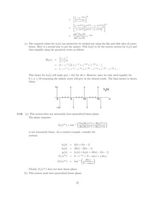
5.7. (a)
H(z) =
z−2
(1 − 1
2 z−1)(1 − 3z−1)
, stable, so the ROC is 1
2 |z| 3
29](https://image.slidesharecdn.com/manualsolucoesexextras-210505182102/85/Manual-solucoes-ex_extras-50-320.jpg)
![x[n] = u[n] ⇔ X(z) =
1
1 − z−1
, |z| 1
Y (z) = X(z)H(z) =
4
5
1 − 1
2 z−1
+
1
5
1 − 3z−1
−
1
1 − z−1
, 1 |z| 3
y[n] =
4
5
1
2
n
u[n] −
1
5
(3)n
u[−n − 1] − u[n]
(b) ROC includes z = ∞ so h[n] is causal. Since both h[n] and x[n] are 0 for n 0, we know that y[n]
is also 0 for n 0
H(z) =
Y (z)
X(z)
=
z−2
1 − 7
2 z−1 + 3
2 z−2
Y (z) −
7
2
z−1
Y (z) +
3
2
z−2
Y (z) = z−2
X(z)
y[n] = x[n − 2] +
7
2
y[n − 1] −
3
2
y[n − 2]
Since y[n] = 0 for n 0, recursion can be done:
y[0] = 0, y[1] = 0, y[2] = 1
(c)
Hi(z) =
1
H(z)
= z2
−
7
2
z +
3
2
, ROC: entire z-plane
hi[n] = δ[n + 2] −
7
2
δ[n + 1] +
3
2
δ[n]
5.8. (a)
X(z) = S(z)(1 − e−8α
z−8
)
H1(z) = 1 − e−8α
z−8
There are 8 zeros at z = e−α
ej π
4 k
for k = 0, . . . , 7
and 8 poles at the origin.
Re
Im
|z|0
1/α
8th order pole
30](https://image.slidesharecdn.com/manualsolucoesexextras-210505182102/85/Manual-solucoes-ex_extras-51-320.jpg)
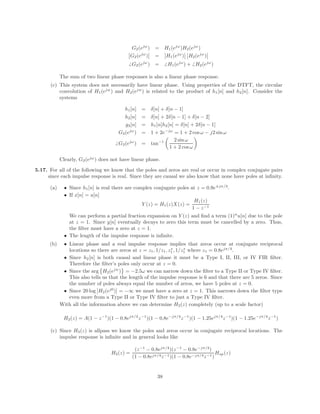
![(b)
Y (z) = H2(z)X(z) = H2(z)H1(z)S(z)
H2(z) =
1
H1(z)
=
1
1 − e−8αz−8
|z| e−α
stable and causal, |z| e−α
not causal or stable
(c) Only the causal h2[n] is stable, therefore only it can be used to
recover s[n].
h[n] =
e−αn
, n = 0, 8, 16, . . .
0, otherwise
(d)
s[n] = δ[n] ⇒ x[n] = δ[n] − e−8α
δ[n − 8]
x[n] ∗ h2[n] = δ[n] − e−8α
δ[n − 8]
+ e−8α
(δ[n − 8] − e−8α
δ[n − 16])
+ e−16α
(δ[n − 16] − e−8α
δ[n − 32]) + · · ·
= δ[n]
5.9.
h[n] =
1
2
n
u[n] +
1
3
n
u[n]
(a)
H(z) =
1
1 − 1
2 z−1
+
1
1 − 1
3 z−1
=
2 − 5
6 z−1
1 − 5
6 z−1 + 1
6 z−2
, |z|
1
2
Since h[n], x[n] = 0 for n 0 we can assume initial rest conditions.
y[n] =
5
6
y[n − 1] −
1
6
y[n − 2] + 2x[n] −
5
6
x[n − 1]
(b)
h1[n] =
h[n], n ≤ 109
0, n 109
(c)
H(z) =
Y (z)
X(z)
=
N−1
X
m=0
h[m]z−m
, N = 109
+ 1
y[n] =
N−1
X
m=0
h[m]x[n − m]
31](https://image.slidesharecdn.com/manualsolucoesexextras-210505182102/85/Manual-solucoes-ex_extras-52-320.jpg)
![(d) For IIR, we have 4 multiplies and 3 adds per output point. This gives us a total of 4N multiplies
and 3N adds. So, IIR grows with order N. For FIR, we have N multiplies and N − 1 adds for the
nth
output point, so this configuration has order N2
.
5.10. (a)
20 log10 |H(ej(π/5)
)| = ∞ ⇒ pole at ej(π/5)
20 log10 |H(ej(2π/5)
)| = −∞ ⇒ zero at ej(2π/5)
Resonance at ω = 3π
5 ⇒ pole inside unit circle
here.
Since the impulse response is real, the poles and zeros must be in
conjugate pairs. The remaining 2 zeros are at zero (the number of poles always equals
the number of zeros).
Re
Im
(b) Since H(z) has poles, we know h[n] is IIR.
(c) Since h[n] is causal and IIR, it cannot be symmetric, and thus
cannot have linear phase.
(d) Since there is a pole at |z| = 1, the ROC does not include the unit
circle. This means the system is not stable.
5.11. Convolving two symmetric sequences yields
another symmetric sequence. A symmetric sequence convolved with an
antisymmetric sequence gives an antisymmetric sequence. If you
convolve two antisymmetric sequences, you will get a symmetric
sequence.
A : h1[n] ∗ h2[n] ∗ h3[n] = (h1[n] ∗ h2[n]) ∗ h3[n]
h1[n] ∗ h2[n] is symmetric about n = 3, (−1 ≤ n ≤ 7)
(h1[n] ∗ h2[n]) ∗ h3[n] is antisymmetric about n = 3, (−3 ≤ n ≤ 9)
Thus, system A has generalized linear phase
B : (h1[n] ∗ h2[n]) + h3[n]
h1[n] ∗ h2[n] is symmetric about n = 3, as we noted above.
Adding h3[n] to this sequence will destroy all symmtery, so this does not have generalized linear phase.
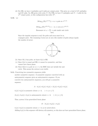
32](https://image.slidesharecdn.com/manualsolucoesexextras-210505182102/85/Manual-solucoes-ex_extras-53-320.jpg)

![(b) A generalized linear phase system has zeros and poles at z = 1, −1, 0 or
∞ or in conjugate reciprocal pairs.
H2(z) =
(1 − 0.5z−1
)
(1 − 0.64z−2)(1 + 1
4 z−2)
Re
Im
3rd order zero
1/2
−(1/2)j
(1/2)j
−4/5 4/5
Hlin(z) = (1 + 1
4 z−2
)(1 + 4z−2
)
Re
Im
4th order pole
−(1/2)j
(1/2)j
−2j
2j
5.13. The input x[n] in the frequency domain looks like
ω
−π −0.5π −0.4π 0 0.4π 0.5π π
(10π) (10π)
5
X(e
jω
)
while the corresponding output y[n] looks like
34](https://image.slidesharecdn.com/manualsolucoesexextras-210505182102/85/Manual-solucoes-ex_extras-55-320.jpg)
![ω
−π −0.3π 0 0.3π π
10e
−j10ω
Y(e
jω
)
Therefore, the filter must be
ω
−π −0.3π 0 0.3π π
2e
−j10ω
H(e
jω
)
In the time domain this is
h[n] =
2 sin[0.3π(n − 10)]
π(n − 10)
5.14. (a)
Property Applies? Comments
Stable No For a stable, causal system, all poles must be
inside the unit circle.
IIR Yes The system has poles at locations other than
z = 0 or z = ∞.
FIR No FIR systems can only have poles at z = 0 or
z = ∞.
Minimum No Minimum phase systems have all poles and zeros
Phase located inside the unit circle.
Allpass No Allpass systems have poles and zeros in conjugate
reciprocal pairs.
Generalized Linear Phase No The causal generalized linear phase systems
presented in this chapter are FIR.
Positive Group Delay for all w No This system is not in the appropriate form.
(b)
35](https://image.slidesharecdn.com/manualsolucoesexextras-210505182102/85/Manual-solucoes-ex_extras-56-320.jpg)
![Property Applies? Comments
Stable Yes The ROC for this system function,
|z| 0, contains the unit circle.
(Note there is 7th order pole at z = 0).
IIR No The system has poles only at z = 0.
FIR Yes The system has poles only at z = 0.
Minimum No By definition, a minimum phase system must
Phase have all its poles and zeros located
inside the unit circle.
Allpass No Note that the zeros on the unit circle will
cause the magnitude spectrum to drop zero at
certain frequencies. Clearly, this system is
not allpass.
Generalized Linear Phase Yes This is the pole/zero plot of a type II FIR
linear phase system.
Positive Group Delay for all w Yes This system is causal and linear phase.
Consequently, its group delay is a positive
constant.
(c)
Property Applies? Comments
Stable Yes All poles are inside the unit circle. Since
the system is causal, the ROC includes the
unit circle.
IIR Yes The system has poles at locations other than
z = 0 or z = ∞.
FIR No FIR systems can only have poles at z = 0 or
z = ∞.
Minimum No Minimum phase systems have all poles and zeros
Phase located inside the unit circle.
Allpass Yes The poles inside the unit circle have
corresponding zeros located at conjugate
reciprocal locations.
Generalized Linear Phase No The causal generalized linear phase systems
presented in this chapter are FIR.
Positive Group Delay for all w Yes Stable allpass systems have positive group delay
for all w.
5.15. (a) Yes.
By the region of convergence we know there are no poles at z = ∞ and it therefore must be causal.
Another way to see this is to use long division to write H1(z) as
H1(z) =
1 − z−5
1 − z−1
= 1 + z−1
+ z−2
+ z−3
+ z−4
, |z| 0
(b) h1[n] is a causal rectangular pulse of length 5. If we convolve h1[n] with another causal rectangular
pulse of length N we will get a triangular pulse of length N + 5 − 1 = N + 4. The triangular pulse
is symmetric around its apex and thus has linear phase. To make the triangular pulse g[n] have at
least 9 nonzero samples we can choose N = 5 or let h2[n] = h1[n].
Proof:
G(ejω
) = H1(ejω
)H2(ejω
) = H2
1 (ejω
)
36](https://image.slidesharecdn.com/manualsolucoesexextras-210505182102/85/Manual-solucoes-ex_extras-57-320.jpg)
![=
1 − e−j5ω
1 − e−jω
2
=
e−jω5/2
ejω5/2
− e−jω5/2
e−jω/2 ejω/2 − e−jω/2
#2
=
sin2
(5ω/2)
sin2
(ω/2)
e−j4ω
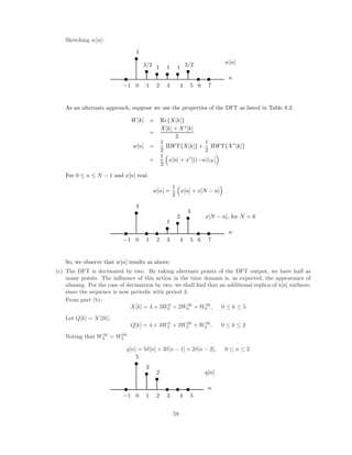
(c) The required values for h3[n] can intuitively be worked out using the flip and slide idea of convo-
lution. Here is a second way to get the answer. Pick h3[n] to be the inverse system for h1[n] and
then simplify using the geometric series as follows.
H3(z) =
1 − z−1
1 − z−5
= (1 − z−1
)
1 + z−5
+ z−10
+ z−15
+ · · ·
= 1 − z−1
+ z−5
− z−6
+ z−10
− z−11
+ z−15
− z−16
+ · · ·
This choice for h3[n] will make q[n] = δ[n] for all n. However, since we only need equality for
0 ≤ n ≤ 19 truncating the infinite series will give us the desired result. The final answer is shown
below.
n
0 5 10 15
1
−1
h
3
[n]
5.16. (a) This system does not necessarily have generalized linear phase.
The phase response,
G1(ejω
) = tan−1
Im(H1(ejω
) + H2(ejω
))
Re(H1(ejω) + H2(ejω))
is not necessarily linear. As a counter-example, consider the
systems
h1[n] = δ[n] + δ[n − 1]
h2[n] = 2δ[n] − 2δ[n − 1]
g1[n] = h1[n] + h2[n] = 3δ[n] − δ[n − 1]
G1(ejω
) = 3 − e−jω
= 3 − cos ω + j sin ω
6 G1(ejω
) = tan−1
sin ω
3 − cos ω
Clearly, G1(ejω
) does not have linear phase.
(b) This system must have generalized linear phase.
37](https://image.slidesharecdn.com/manualsolucoesexextras-210505182102/85/Manual-solucoes-ex_extras-58-320.jpg)


![6 G2(ejω
) = 6 H1(ejω
) + 6 H2(ejω
)
The sum of two linear phase responses is also a linear phase response.
(c) This system does not necessarily have linear phase. Using properties of the DTFT, the circular
convolution of H1(ejw
) and H2(ejw
) is related to the product of h1[n] and h2[n]. Consider the
systems
h1[n] = δ[n] + δ[n − 1]
h2[n] = δ[n] + 2δ[n − 1] + δ[n − 2]
g3[n] = h1[n]h2[n] = δ[n] + 2δ[n − 1]
G3(ejω
) = 1 + 2e−jω
= 1 + 2 cosω − j2 sin ω
6 G3(ejω
) = tan−1
2 sin ω
1 + 2 cosω
Clearly, G3(ejω
) does not have linear phase.
5.17. For all of the following we know that the poles and zeros are real or occur in complex conjugate pairs
since each impulse response is real. Since they are causal we also know that none have poles at infinity.
(a) • Since h1[n] is real there are complex conjugate poles at z = 0.9e±jπ/3
.
• If x[n] = u[n]
Y (z) = H1(z)X(z) =
H1(z)
1 − z−1
We can perform a partial fraction expansion on Y (z) and find a term (1)n
u[n] due to the pole
at z = 1. Since y[n] eventually decays to zero this term must be cancelled by a zero. Thus,
the filter must have a zero at z = 1.
• The length of the impulse response is infinite.
(b) • Linear phase and a real impulse response implies that zeros occur at conjugate reciprocal
locations so there are zeros at z = z1, 1/z1, z∗
1, 1/z∗
1 where z1 = 0.8ejπ/4
.
• Since h2[n] is both causal and linear phase it must be a Type I, II, III, or IV FIR filter.
Therefore the filter’s poles only occur at z = 0.
• Since the arg
H2(ejw
)
= −2.5ω we can narrow down the filter to a Type II or Type IV filter.
This also tells us that the length of the impulse response is 6 and that there are 5 zeros. Since
the number of poles always equal the number of zeros, we have 5 poles at z = 0.
• Since 20 log](https://image.slidesharecdn.com/manualsolucoesexextras-210505182102/85/Manual-solucoes-ex_extras-71-320.jpg)


![5.18. (a) To be rational, X(z) must be of the form
X(z) =
b0
a0
M
Y
k=1
(1 − ckz−1
)
N
Y
k=1
(1 − dkz−1
)
Because x[n] is real, its zeros must appear in conjugate pairs. Consequently, there are two more
zeros, at z = 1
2 e−jπ/4
, and z = 1
2 e−j3π/4
. Since x[n] is zero outside 0 ≤ n ≤ 4, there are only four
zeros (and poles) in the system function. Therefore, the system function can be written as
X(z) =
1 −
1
2
ejπ/4
z−1
1 −
1
2
ej3π/4
z−1
1 −
1
2
e−jπ/4
z−1
1 −
1
2
e−j3π/4
z−1
Clearly, X(z) is rational.
(b) A sketch of the pole-zero plot for X(z) is shown below. Note that the ROC for X(z) is |z| 0.
Re
Im
4th order pole
X(z)
(c) A sketch of the pole-zero plot for Y (z) is shown below. Note that the ROC for Y(z) is |z| 1
2 .
Re
Im
4th order zero
Y(z)
5.19. • Since x[n] is real the poles zeros come in complex conjugate pairs.
• From (1) we know there are no poles except at zero or infinity.
• From (3) and the fact that x[n] is finite we know that the signal has generalized linear phase.
• From (3) and (4) we have α = 2. This and the fact that there are no poles in the finite
plane except the five at zero (deduced from (1) and (2)) tells us the form of X(z) must be
X(z) = x[−1]z + x[0] + x[1]z−1
+ x[2]z−2
+ x[3]z−3
+ x[4]z−4
+ x[5]z−5
The phase changes by π at ω = 0 and π so there must be a zero on the unit circle at z = ±1. The
zero at z = 1 tells us
P
x[n] = 0. The zero at z = −1 tells us
P
(−1)n
x[n] = 0.
We can also conclude x[n] must be a Type III filter since the length of x[n] is odd and there is a
zero at both z = ±1. x[n] must therefore be antisymmetric around n = 2 and x[2] = 0.
• From (5) and Parseval’s theorem we have
P
|x[n]|2
= 28.
39](https://image.slidesharecdn.com/manualsolucoesexextras-210505182102/85/Manual-solucoes-ex_extras-76-320.jpg)
![• From (6)
y[0] =
1
2π
Z π
−π
Y (ejω
)dω = 4
= x[n] ∗ u[n] |n=0 = x[−1] + x[0]
y[1] =
1
2π
Z π
−π
Y (ejω
)ejw
dω = 6
= x[n] ∗ u[n] |n=1 = x[−1] + x[0] + x[1]
• The conclusion from (7) that
P
(−1)n
x[n] = 0 we already derived earlier.
• Since the DTFT {xe[n]} = Re
X(ejω
)
we have
x[5] + x[−5]
2
= −
3
2
x[5] = −3 + x[−5]
x[5] = −3
Summarizing the above we have the following (dependent) equations
(1) x[−1] + x[0] + x[1] + x[2] + x[3] + x[4] + x[5] = 0
(2) −x[−1] + x[0] − x[1] + x[2] − x[3] + x[4] − x[5] = 0
(3) x[2] = 0
(4) x[−1] = −x[5]
(5) x[0] = −x[4]
(6) x[1] = −x[3]
(7) x[−1]2
+ x[0]2
+ x[1]2
+ x[2]2
+ x[3]2
+ x[4]2
+ x[5]2
= 28
(8) x[−1] + x[0] = 4
(9) x[−1] + x[0] + x[1] = 6
(10) x[5] = −3
x[n] is easily obtained from solving the equations in the following order: (3),(10),(4),(8),(5),(9), and (6).
n
−1 0 1 2
3 4 5
3
1
2
−2
−1
−3
x[n]
40](https://image.slidesharecdn.com/manualsolucoesexextras-210505182102/85/Manual-solucoes-ex_extras-77-320.jpg)

The document provides solutions to problems from a discrete-time signal processing textbook. It includes: 1) Solutions to convolution problems graphically representing signals and their convolution. 2) Derivations of impulse responses from system functions using the z-transform. 3) Analyses of signals as eigenfunctions and determining if systems are linear and time-invariant. 4) Solutions involving filtering, modulation, and determining system properties from inputs and outputs.


![[4] num integration](https://cdn.slidesharecdn.com/ss_thumbnails/4numintegration-120403041412-phpapp02-thumbnail.jpg?width=640&height=640&fit=bounds)