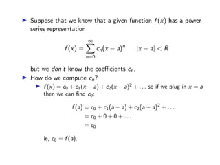
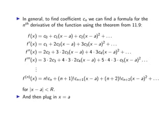
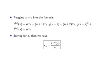
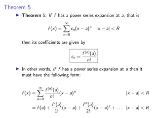
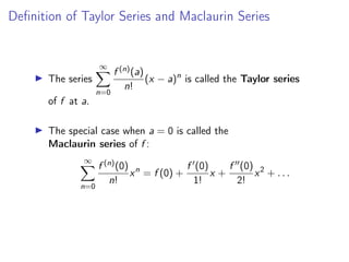
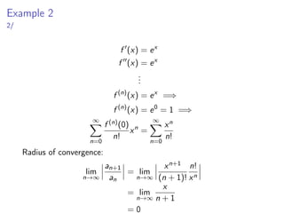
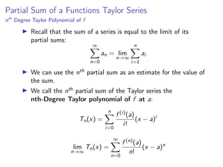
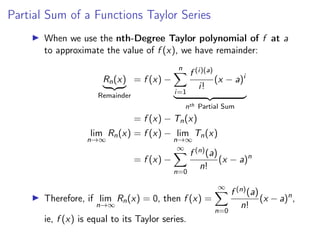
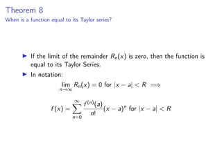
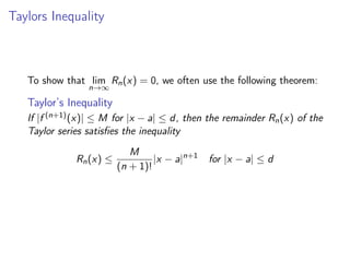
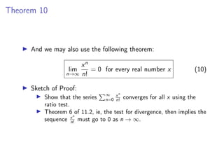
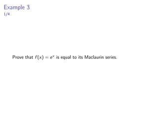
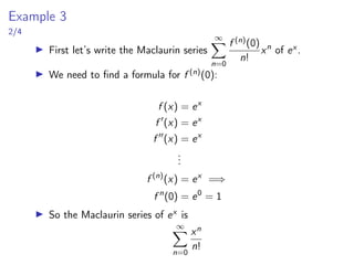
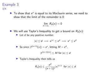
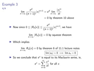
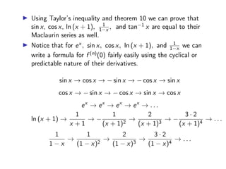
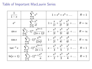
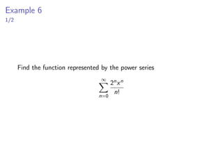
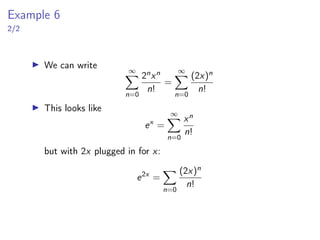
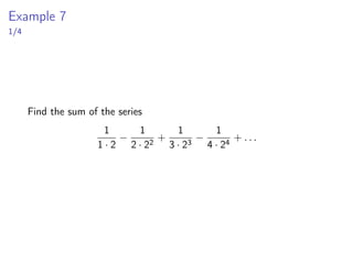
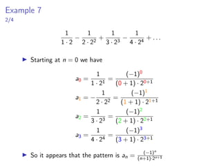
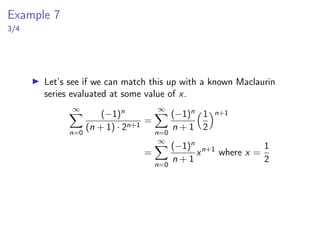
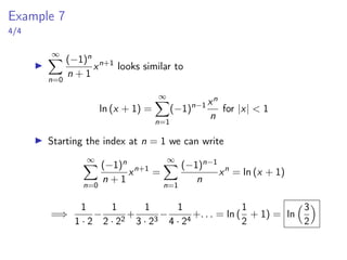
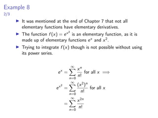
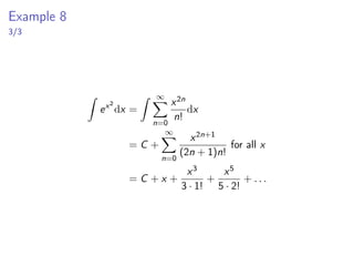
Numerical Methods was a core subject for Electrical & Electronics Engineering, Based On Anna University Syllabus. The Whole Subject was there in this document.
Share with it ur friends & Follow me for more updates.!
Mathematics (from Greek μάθημα máthēma, “knowledge, study, learning”) is the study of topics such as quantity (numbers), structure, space, and change. There is a range of views among mathematicians and philosophers as to the exact scope and definition of mathematics
A numerical method to solve fractional Fredholm-Volterra integro-differential...OctavianPostavaru
The Goolden ratio is famous for the predictability it provides both in the microscopic world as well as in the dynamics of macroscopic structures of the universe. The extension of the Fibonacci series to the Fibonacci polynomials gives us the opportunity to use this powerful tool in the study of Fredholm-Volterra integro-differential equations. In this paper, we define a new hybrid fractional function consisting of block-pulse functions and Fibonacci polynomials (FHBPF). For this, in the Fibonacci polynomials we perform the transformation $x\to x^{\alpha}$, with $\alpha$ a real parameter. In the method developed in this paper, we propose that the unknown function $D^{\alpha}f(x)$ be written as a linear combination of FHBPF. We consider the fractional derivative $D^{\alpha}$ in the Caputo sense. Using theoretical considerations, we can write both the function $f(x)$ and other involved functions of type $D^{\beta}f(x)$ on the same basis. For this operation, we have to define an integral operator of Riemann-Liouville type associated to FHBPF, and with the help of hypergeometric functions, we can express this operator exactly. All these ingredients together with the collocation in the Newton-Cotes nodes transform the integro-differential equation into an algebraic system that we solve by applying Newton's iterative method. We conclude the paper with some examples to demonstrate that the proposed method is simple to implement and accurate. There are situations when by simply considering $\alpha\ne1$, we obtain an improvement in accuracy by 12 orders of magnitude.
Palestine last event orientationfvgnh .pptxRaedMohamed3
An EFL lesson about the current events in Palestine. It is intended to be for intermediate students who wish to increase their listening skills through a short lesson in power point.
We all have good and bad thoughts from time to time and situation to situation. We are bombarded daily with spiraling thoughts(both negative and positive) creating all-consuming feel , making us difficult to manage with associated suffering. Good thoughts are like our Mob Signal (Positive thought) amidst noise(negative thought) in the atmosphere. Negative thoughts like noise outweigh positive thoughts. These thoughts often create unwanted confusion, trouble, stress and frustration in our mind as well as chaos in our physical world. Negative thoughts are also known as “distorted thinking”.
Welcome to TechSoup New Member Orientation and Q&A (May 2024).pdfTechSoup
In this webinar you will learn how your organization can access TechSoup's wide variety of product discount and donation programs. From hardware to software, we'll give you a tour of the tools available to help your nonprofit with productivity, collaboration, financial management, donor tracking, security, and more.
The Indian economy is classified into different sectors to simplify the analysis and understanding of economic activities. For Class 10, it's essential to grasp the sectors of the Indian economy, understand their characteristics, and recognize their importance. This guide will provide detailed notes on the Sectors of the Indian Economy Class 10, using specific long-tail keywords to enhance comprehension.
For more information, visit-www.vavaclasses.com
This is a presentation by Dada Robert in a Your Skill Boost masterclass organised by the Excellence Foundation for South Sudan (EFSS) on Saturday, the 25th and Sunday, the 26th of May 2024.
He discussed the concept of quality improvement, emphasizing its applicability to various aspects of life, including personal, project, and program improvements. He defined quality as doing the right thing at the right time in the right way to achieve the best possible results and discussed the concept of the "gap" between what we know and what we do, and how this gap represents the areas we need to improve. He explained the scientific approach to quality improvement, which involves systematic performance analysis, testing and learning, and implementing change ideas. He also highlighted the importance of client focus and a team approach to quality improvement.
4. ▶ Suppose that we know that a given function f (x) has a power
series representation
f (x) =
∞
X
n=0
cn(x − a)n
|x − a| < R
but we don’t know the coefficients cn.
▶ How do we compute cn?
▶ f (x) = c0 + c1(x − a) + c2(x − a)2
+ . . . so if we plug in x = a
then we can find c0:
f (a) = c0 + c1(a − a) + c2(a − a)2
+ . . .
= c0 + 0 + 0 + . . .
= c0
ie, c0 = f (a).
5. ▶ In general, to find coefficient cn we can find a formula for the
nth derivative of the function using the theorem from 11.9:
f (x) = c0 + c1(x − a) + c2(x − a)2
+ . . .
f ′
(x) = c1 + 2c2(x − a) + 3c3(x − a)2
+ . . .
f ′′
(x) = 2c2 + 3 · 2c3(x − a) + 4 · 3c4(x − a)2
+ . . .
f ′′′
(x) = 3 · 2c3 + 4 · 3 · 2c4(x − a) + 5 · 4 · 3 · c5(x − a)2
. . .
.
.
.
f (n)
(x) = n!cn + (n + 1)!cn+1(x − a) + (n + 2)!cn+2(x − a)2
+ . . .
for |x − a| < R.
▶ And then plug in x = a
6. ▶ Plugging x = a into the formula:
f (n)
(x) = n!cn + (n + 1)!cn+1(x − a) + (n + 2)!cn+2(x − a)2
+ . . .
f (n)
(a) = n!cn
▶ Solving for cn then we have
cn =
f (n)(a)
n!
7. Theorem 5
▶ Theorem 5: If f has a power series expansion at a, that is
f (x) =
∞
X
n=0
cn(x − a)n
|x − a| < R
then its coefficients are given by
cn =
f (n)(a)
n!
▶ In other words, if f has a power series expansion at a then it
must have the following form:
f (x) =
∞
X
n=0
f (n)(a)
n!
(x − a)n
|x − a| < R
= f (a) +
f ′(a)
1!
(x − a) +
f ′′(a)
2!
(x − a)2
+ . . . |x − a| < R
8. Definition of Taylor Series and Maclaurin Series
▶ The series
∞
X
n=0
f (n)(a)
n!
(x − a)n
is called the Taylor series
of f at a.
▶ The special case when a = 0 is called the
Maclaurin series of f :
∞
X
n=0
f (n)(0)
n!
xn
= f (0) +
f ′(0)
1!
x +
f ′′(0)
2!
x2
+ . . .
9. Remark
▶ It is not always guaranteed that f (x) is equal to the sum of its
Taylor series because not all functions have a power series
representation at a.
▶ Nonetheless, we can compute the Taylor series of any
differentiable function by using the theorem and formula above.
13. Example 2
1/
Find the Maclaurin series and radius of convergence for the function
f (x) = ex
14. Example 2
2/
f ′
(x) = ex
f ′′
(x) = ex
.
.
.
f (n)
(x) = ex
=⇒
f (n)
(x) = e0
= 1 =⇒
∞
X
n=0
f (n)(0)
n!
xn
=
∞
X
n=0
xn
n!
Radius of convergence:
lim
n→∞
27. When is a Function Represented by its Taylor
Series?
28. Partial Sum of a Functions Taylor Series
nth
Degree Taylor Polynomial of f
▶ Recall that the sum of a series is equal to the limit of its
partial sums:
∞
X
n=0
an = lim
n→∞
n
X
i=1
ai
▶ We can use the nth partial sum as an estimate for the value of
the sum.
▶ We call the nth partial sum of the Taylor series the
nth-Degree Taylor polynomial of f at a:
Tn(x) =
n
X
i=0
f (i)(a)
i!
(x − a)i
lim
n→∞
Tn(x) =
∞
X
n=0
f (n)(a)
n!
(x − a)n
29. Partial Sum of a Functions Taylor Series
▶ When we use the nth-Degree Taylor polynomial of f at a
to approximate the value of f (x), we have remainder:
Rn(x)
| {z }
Remainder
= f (x) −
n
X
i=1
f (i)(a)
i!
(x − a)i
| {z }
nth Partial Sum
= f (x) − Tn(x)
lim
n→∞
Rn(x) = f (x) − lim
n→∞
Tn(x)
= f (x) −
∞
X
n=0
f (n)(a)
n!
(x − a)n
▶ Therefore, if lim
n→∞
Rn(x) = 0, then f (x) =
∞
X
n=0
f (n)(a)
n!
(x − a)n
,
ie, f (x) is equal to its Taylor series.
30. Theorem 8
When is a function equal to its Taylor series?
▶ If the limit of the remainder Rn(x) is zero, then the function is
equal to its Taylor Series.
▶ In notation:
lim
n→∞
Rn(x) = 0 for |x − a| < R =⇒
f (x) =
∞
X
n=0
f (n)(a)
n!
(x − a)n
for |x − a| < R
31. Taylors Inequality
To show that lim
n→∞
Rn(x) = 0, we often use the following theorem:
Taylor’s Inequality
If |f (n+1)(x)| ≤ M for |x − a| ≤ d, then the remainder Rn(x) of the
Taylor series satisfies the inequality
Rn(x) ≤
M
(n + 1)!
|x − a|n+1
for |x − a| ≤ d
32. Theorem 10
▶ And we may also use the following theorem:
lim
n→∞
xn
n!
= 0 for every real number x (10)
▶ Sketch of Proof:
▶ Show that the series
P∞
n=0
xn
n! converges for all x using the
ratio test.
▶ Theorem 6 of 11.2, ie, the test for divergence, then implies the
sequence xn
n! must go to 0 as n → ∞.
34. Example 3
2/4
▶ First let’s write the Maclaurin series
∞
X
n=0
f (n)(0)
n!
xn
of ex .
▶ We need to find a formula for f (n)(0):
f (x) = ex
f ′
(x) = ex
f ′′
(x) = ex
.
.
.
f (n)
(x) = ex
=⇒
f n
(0) = e0
= 1
▶ So the Maclaurin series of ex is
∞
X
n=0
xn
n!
35. Example 3
3/4
▶ To show that ex is equal to its Maclaurin series, we need to
show that the limit of the remainder is 0:
lim
n→∞
Rn(x) = 0
▶ We will use Taylor’s Inequality to get a bound on Rn(x):
▶ Let d be any positive number.
|x| ≤ d =⇒ e|x|
≤ ed
=⇒ ex
≤ ed
▶ So since |f (n+1)
(x)| = ex
, letting M = ed
,
|f (n+1)(x)
| ≤ M for |x| ≤ d
▶ Taylor’s Inequality then tells us
Rn(x) ≤
ed
(n + 1)!
|x|n+1
for |x| ≤ d
36. Example 3
4/4
lim
n→∞
ed
(n + 1)!
|x|n+1
= ed
lim
n→∞
|x|n
n!
= 0 by theorem 10 above
▶ Now since 0 ≤ |Rn(x)| ≤
ed
(n + 1)!
|x|n+1
, we have
lim
n→∞
|Rn(x)| = 0 by squeeze theorem
▶ Which implies
lim
n→∞
Rn(x) = 0 by theorem 6 of 11.1 lecture notes
lim |an| = 0 =⇒ lim an = 0
▶ So we conclude that ex is equal to its Maclaurin series, ie,
ex
=
∞
X
n=0
xn
n!
for all x
37.
38. ▶ Using Taylor’s inequality and theorem 10 we can prove that
sin x, cos x, ln (x + 1), 1
1−x , and tan−1 x are equal to their
Maclaurin series as well.
▶ Notice that for ex , sin x, cos x, ln (x + 1), and 1
1−x we can
write a formula for f (n)(0) fairly easily using the cyclical or
predictable nature of their derivatives.
sin x → cos x → − sin x → − cos x → sin x
cos x → − sin x → − cos x → sin x → cos x
ex
→ ex
→ ex
→ ex
→ . . .
ln (x + 1) →
1
x + 1
→ −
1
(x + 1)2
→
2
(x + 1)3
→ −
3 · 2
(x + 1)4
→ . . .
1
1 − x
→
1
(1 − x)2
→
2
(1 − x)3
→
3 · 2
(1 − x)4
→ . . .
39. Table of Important MacLaurin Series
1
1 − x
∞
X
n=0
xn
1 + x2 + x3 + . . . R = 1
ex
∞
X
n=0
xn
n!
1 +
x
1!
+
x2
2!
+
x3
3!
+ . . . R = ∞
sin x
∞
X
n=0
(−1)n x2n+1
(2n + 1)!
x −
x3
3!
+
x5
5!
−
x7
6!
+ . . . R = ∞
cos x
∞
X
n=0
(−1)n x2n
(2n)!
1 −
x2
2!
+
x4
4!
−
x6
6!
+ . . . R = ∞
tan−1 x
∞
X
n=0
(−1)n x2n+1
2n + 1
x −
x3
3
+
x5
5
−
x7
7
+ . . . R = 1
ln(x + 1)
∞
X
n=1
(−1)n−1 xn
n
x −
x2
2
+
x3
3
−
x4
4
+ . . . R = 1
42. Example 5
2/3
(a) We know
cos x =
∞
X
n=0
(−1)n x2n
(2n)!
for all values of x. So multiplying both sides by x we have
x cos x = x
∞
X
n=0
(−1)n x2n
(2n)!
=
∞
X
n=0
(−1)n x2n+1
(2n)!
for all x
43. Example 5
3/3
(b) We know that
ln (1 + x) =
∞
X
n=0
(−1)n−1 xn
n
for |x| < 1
So plugging 3x2 in for x on both sides we get
ln(1 + 3x2
) =
∞
X
n=0
(−1)n−1 (3x2)n
n
=
∞
X
n=0
(−1)n−1 3n
n
x2n
for |3x2| < 1, ie, |x| < 1
√
3
.
45. Example 6
2/2
▶ We can write
∞
X
n=0
2nxn
n!
=
∞
X
n=0
(2x)n
n!
▶ This looks like
ex
=
∞
X
n=0
xn
n!
but with 2x plugged in for x:
e2x
=
X
n=0
(2x)n
n!
46. Example 7
1/4
Find the sum of the series
1
1 · 2
−
1
2 · 22
+
1
3 · 23
−
1
4 · 24
+ . . .
47. Example 7
2/4
1
1 · 2
−
1
2 · 22
+
1
3 · 23
−
1
4 · 24
+ . . .
▶ Starting at n = 0 we have
a0 =
1
1 · 21
=
(−1)0
(0 + 1) · 20+1
a1 = −
1
2 · 22
=
(−1)1
(1 + 1) · 21+1
a2 =
1
3 · 23
=
(−1)2
(2 + 1) · 22+1
a3 =
1
4 · 24
=
(−1)3
(3 + 1) · 23+1
▶ So it appears that the pattern is an = (−1)n
(n+1)·2n+1
48. Example 7
3/4
▶ Let’s see if we can match this up with a known Maclaurin
series evaluated at some value of x.
∞
X
n=0
(−1)n
(n + 1) · 2n+1
=
∞
X
n=0
(−1)n
n + 1
1
2
n+1
=
∞
X
n=0
(−1)n
n + 1
xn+1
where x =
1
2
49. Example 7
4/4
▶
∞
X
n=0
(−1)n
n + 1
xn+1
looks similar to
ln (x + 1) =
∞
X
n=1
(−1)n−1 xn
n
for |x| 1
▶ Starting the index at n = 1 we can write
∞
X
n=0
(−1)n
n + 1
xn+1
=
∞
X
n=1
(−1)n−1
n
xn
= ln (x + 1)
=⇒
1
1 · 2
−
1
2 · 22
+
1
3 · 23
−
1
4 · 24
+. . . = ln (
1
2
+ 1) = ln
3
2
51. Example 8
2/3
▶ It was mentioned at the end of Chapter 7 that not all
elementary functions have elementary derivatives.
▶ The function f (x) = ex2
is an elementary function, as it is
made up of elementary functions ex and x2.
▶ Trying to integrate f (x) though is not possible without using
its power series.
ex
=
∞
X
n=0
xn
n!
for all x =⇒
ex2
=
∞
X
n=0
(x2)n
n!
for all x
=
∞
X
n=0
x2n
n!
52. Example 8
3/3
Z
ex2
dx =
Z ∞
X
n=0
x2n
n!
dx
= C +
∞
X
n=0
x2n+1
(2n + 1)n!
for all x
= C + x +
x3
3 · 1!
+
x5
5 · 2!
+ . . .
53. Just for Fun
▶ What if we had tried to use substitution?
s = x2, ds = 2xdx =⇒ dx = ds
2x = ds
2
√
s
Z
ex2
dx =
Z
es
2
√
s
ds
▶ Now use integration by parts
u = es dv = 1
2
√
s
ds
du = esds v =
√
s
#
Z
es
2
√
s
ds = es√
s −
Z
√
ses
ds
54. ▶ Integration by parts again:
u = es dv =
√
sds
du = esds v = 2s3/2
3
#
Z
√
ses
ds =
2ess3/2
3
−
Z
2s3/2
3
es
ds
▶ Again
u = es dv = 2s3/2
3 ds
du = esds v = 4s5/2
15
#
Z
2s3/2
3
es
ds =
4ess5/2
15
−
Z
4s5/2
15
es
ds
55. ▶ Imagine we keep going like this. . .forever
▶ Just putting the first three iterations together we have:
Z
ex2
dx = xex2
−
2
3
x3
ex2
+
4
15
x5
ex2
−
8
105
x7
ex2
. . .
=
x −
2
3
x3
+
22
3 · 5
x5
−
23
3 · 5 · 7
x7
+ . . .
ex2
=
x −
2
3
x3
+
22
3 · 5
x5
−
23
3 · 5 · 7
x7
+ . . .
∞
X
n=0
x2n
n!
=
∞
X
n=0
(−2)nx2n+1
Kn
·
∞
X
n=0
x2n
n!
where Kn = (2n − 1) · (2n − 3) · (2n − 5) · . . . · 1.