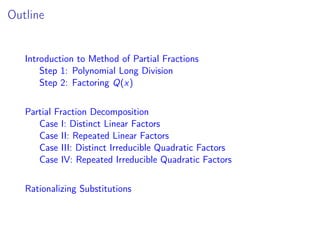
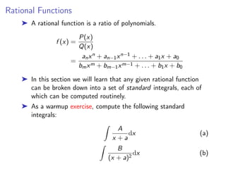
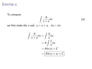
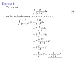
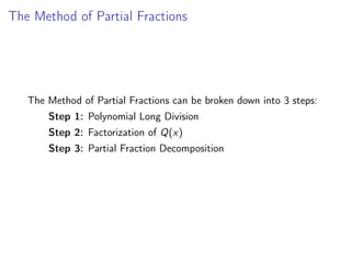
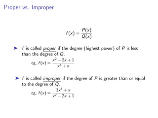
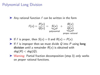
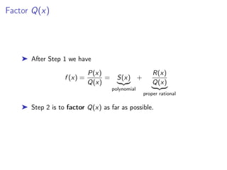
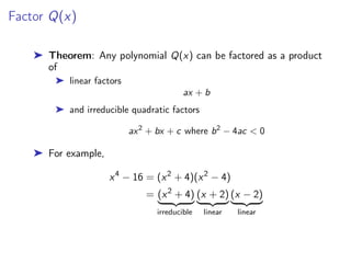
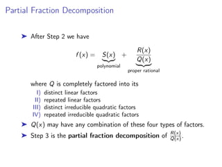
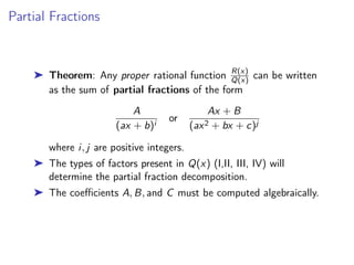
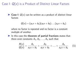
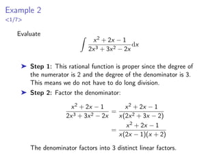
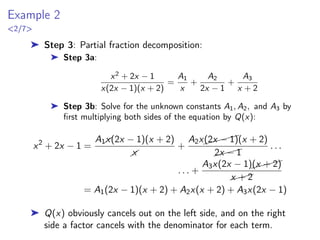
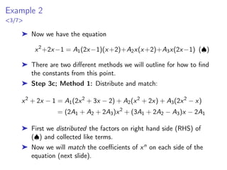
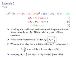
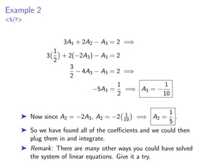
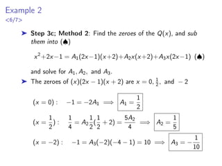
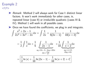
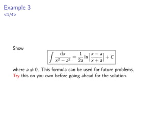
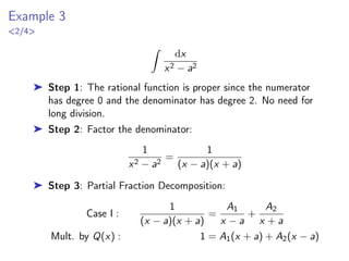
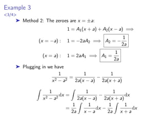
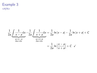
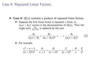
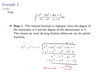
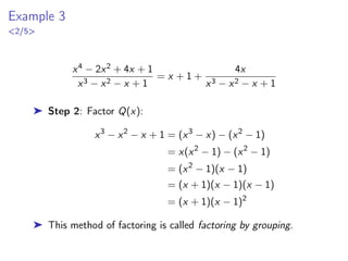
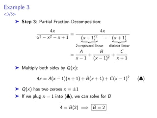
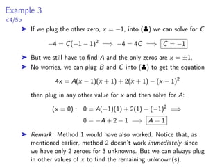
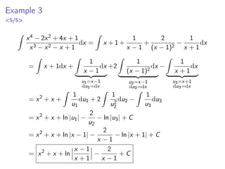
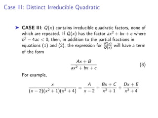
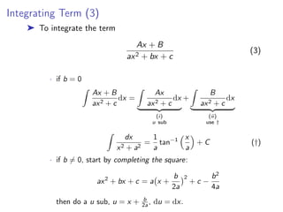
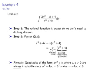
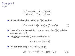
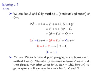
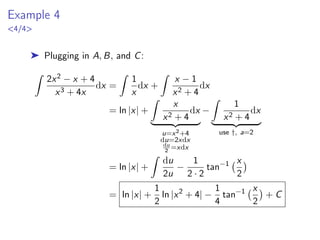
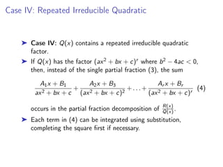
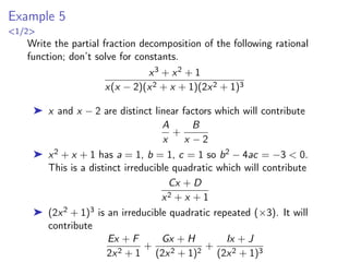
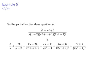
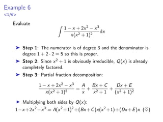
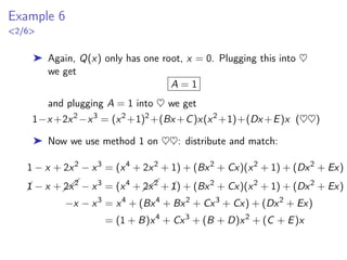
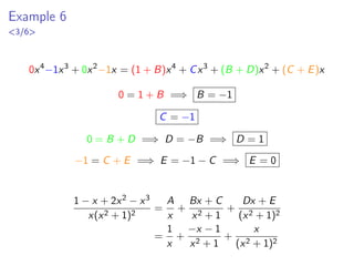
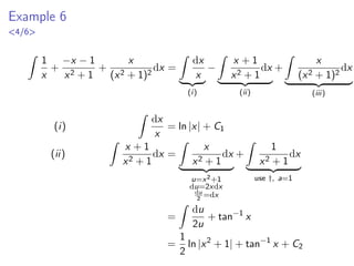
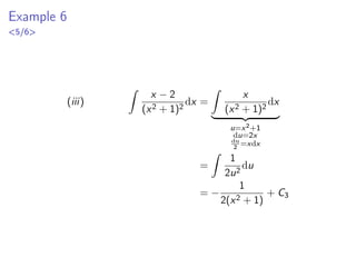
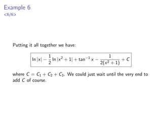
This document discusses the method of partial fractions for integrating rational functions. It begins by introducing rational functions and the goal of breaking them into standard integrals. There are four cases for partial fraction decomposition based on the factors of the denominator: I) distinct linear factors, II) repeated linear factors, III) distinct irreducible quadratic factors, and IV) repeated irreducible quadratic factors. The method involves three steps: 1) polynomial long division, 2) factoring the denominator, and 3) determining the partial fraction decomposition. Examples are provided to demonstrate the technique.

1. Chapter 7: Techniques of Integration
Section 7.4: Integration of Rational Functions by Partial
Fractions
Alea Wittig
SUNY Albany

2. Outline
Introduction to Method of Partial Fractions
Step 1: Polynomial Long Division
Step 2: Factoring Q(x)
Partial Fraction Decomposition
Case I: Distinct Linear Factors
Case II: Repeated Linear Factors
Case III: Distinct Irreducible Quadratic Factors
Case IV: Repeated Irreducible Quadratic Factors
Rationalizing Substitutions

3. Introduction to Method of Partial Fractions

4. Rational Functions
➤ A rational function is a ratio of polynomials.
f (x) =
P(x)
Q(x)
=
anxn + an−1xn−1 + . . . + a1x + a0
bmxm + bm−1xm−1 + . . . + b1x + b0
➤ In this section we will learn that any given rational function
can be broken down into a set of standard integrals, each of
which can be computed routinely.
➤ As a warmup exercise, compute the following standard
integrals:
Z
A
x + a
dx (a)
Z
B
(x + a)2
dx (b)

5. Exercise a
To compute Z
A
x + a
dx (a)
we first make the u sub: u = x + a, du = dx
Z
A
x + a
dx =
Z
A
u
du
= A
Z
1
u
du
= A ln |u| + C
= A ln |x + a| + C

6. Exercise b
To compute Z
B
(x + a)2
dx (b)
we first make the u sub: u = x + a, du = dx
Z
B
(x + a)2
dx =
Z
B
u2
du
= B
Z
1
u2
du
= B
Z
u−2
du
= B
u−2+1
−2 + 1
+ C
= B
u−1
−1
+ C
= −
B
u
+ C = −
B
x + a
+ C

7. The Method of Partial Fractions
The Method of Partial Fractions can be broken down into 3 steps:
Step 1: Polynomial Long Division
Step 2: Factorization of Q(x)
Step 3: Partial Fraction Decomposition

8. Step 1: Polynomial Long Division

9. Proper vs. Improper
f (x) =
P(x)
Q(x)
➤ f is called proper if the degree (highest power) of P is less
than the degree of Q.
eg, f (x) =
x2
− 2x + 1
x3 + x
➤ f is called improper if the degree of P is greater than or equal
to the degree of Q.
eg, f (x) =
3x5
+ x
x2 − 2x + 1

10. Polynomial Long Division
➤ Any rational function f can be written in the form
f (x) =
P(x)
Q(x)
= S(x)
|{z}
polynomial
+
R(x)
Q(x)
| {z }
proper rational
➤ If f is proper, then S(x) = 0 and R(x) = P(x)
➤ If f is improper then we must divide Q into P using long
division until a remainder R(x) is obtained with
deg(R) < deg(Q).
➤ Warning: Partial fraction decomposition (step 3) only works
on proper rational functions.

11. Example 1
Video Example 1

12. Exercise c
As an exercise, use long division to show that
x3 + x
x − 1
= x2
+ x + 2 +
2
x − 1
Use this to compute the integral
Z
x3 + x
x − 1
dx

13. ➤ In example 1 and exercise c we were able to write the rational
function as a sum of standard integrals which were simple to
compute.
➤ If we are not able to integrate after step 1 then move on to
step 2.

14. Step 2: Factoring Q(x)

15. Factor Q(x)
➤ After Step 1 we have
f (x) =
P(x)
Q(x)
= S(x)
|{z}
polynomial
+
R(x)
Q(x)
| {z }
proper rational
➤ Step 2 is to factor Q(x) as far as possible.

16. Factor Q(x)
➤ Theorem: Any polynomial Q(x) can be factored as a product
of
➤ linear factors
ax + b
➤ and irreducible quadratic factors
ax2
+ bx + c where b2
− 4ac < 0
➤ For example,
x4
− 16 = (x2
+ 4)(x2
− 4)
= (x2
+ 4)
| {z }
irreducible
(x + 2)
| {z }
linear
(x − 2)
| {z }
linear

17. Partial Fraction Decomposition

18. Partial Fraction Decomposition
➤ After Step 2 we have
f (x) = S(x)
|{z}
polynomial
+
R(x)
Q(x)
| {z }
proper rational
where Q is completely factored into its
I) distinct linear factors
II) repeated linear factors
III) distinct irreducible quadratic factors
IV) repeated irreducible quadratic factors
➤ Q(x) may have any combination of these four types of factors.
➤ Step 3 is the partial fraction decomposition of R(x)
Q(x).

19. Partial Fractions
➤ Theorem: Any proper rational function R(x)
Q(x) can be written
as the sum of partial fractions of the form
A
(ax + b)i
or
Ax + B
(ax2 + bx + c)j
where i, j are positive integers.
➤ The types of factors present in Q(x) (I,II, III, IV) will
determine the partial fraction decomposition.
➤ The coefficients A, B, and C must be computed algebraically.

20. Case I: Distinct Linear Factors

21. Case I: Q(x) is a Product of Distinct Linear Factors
➤ Case I: Q(x) can be written as a product of distinct linear
factors
Q(x) = (a1x + b1)(a2x + b2) . . . (akx + bk)
where no factor is repeated and no factor is a constant
multiple of another.
➤ In this case the theorem of partial fractions states that
there exist constants A1, A2, . . . , Ak such that
R(x)
Q(x)
=
A1
a1x + b1
+
A2
a2x + b2
+ . . . +
Ak
akx + bk
(1)

22. Example 2
<1/7>
Evaluate Z
x2 + 2x − 1
2x3 + 3x2 − 2x
dx
➤ Step 1: This rational function is proper since the degree of
the numerator is 2 and the degree of the denominator is 3.
This means we do not have to do long division.
➤ Step 2: Factor the denominator:
x2 + 2x − 1
2x3 + 3x2 − 2x
=
x2 + 2x − 1
x(2x2 + 3x − 2)
=
x2 + 2x − 1
x(2x − 1)(x + 2)
The denominator factors into 3 distinct linear factors.

23. Example 2
<2/7>
➤ Step 3: Partial fraction decomposition:
➤ Step 3a:
x2
+ 2x − 1
x(2x − 1)(x + 2)
=
A1
x
+
A2
2x − 1
+
A3
x + 2
➤ Step 3b: Solve for the unknown constants A1, A2, and A3 by
first multiplying both sides of the equation by Q(x):
x2
+ 2x − 1 =
A1
x(2x − 1)(x + 2)
x
+
A2x
(2x − 1)(x + 2)
2x − 1
. . .
. . . +
A3x(2x − 1)
(x + 2)
x + 2
= A1(2x − 1)(x + 2) + A2x(x + 2) + A3x(2x − 1)
➤ Q(x) obviously cancels out on the left side, and on the right
side a factor cancels with the denominator for each term.

24. Example 2
3/7
➤ Now we have the equation
x2
+2x−1 = A1(2x−1)(x+2)+A2x(x+2)+A3x(2x−1) (♠)
➤ There are two different methods we will outline for how to find
the constants from this point.
➤ Step 3c; Method 1: Distribute and match:
x2
+ 2x − 1 = A1(2x2
+ 3x − 2) + A2(x2
+ 2x) + A3(2x2
− x)
= (2A1 + A2 + 2A3)x2
+ (3A1 + 2A2 − A3)x − 2A1
➤ First we distributed the factors on right hand side (RHS) of
(♠) and collected like terms.
➤ Now we will match the coefficients of xn on each side of the
equation (next slide).

25. Example 2
4/7
1x2
+ 2x−1 = (2A1 + A2 + 2A3)x2
+ (3A1 + 2A2 − A3)x + −2A1
2A1 + A2 + 2A3 = 1 (i)
3A1 + 2A2 − A3 = 2 (ii)
−2A1 = −1 (iii)
➤ Matching the coefficients we have formed 3 equations for our
3 unknowns A1, A2, A3. This is called a system of linear
equations.
➤ We can immediately solve (iii) for A1: A1 =
1
2
➤ We could then plug this into (i) to solve for A2 in terms of A3.
2
1
2
+ A2 + 2A3 = 1 =⇒ A2 = −2A3
➤ Now plug A1 = 1
2 and A2 = −2A3 into (ii) (next slide).

26. Example 2
5/7
3A1 + 2A2 − A3 = 2 =⇒
3
1
2
+ 2(−2A3) − A3 = 2
3
2
− 4A3 − A3 = 2 =⇒
−5A3 =
1
2
=⇒ A3 = −
1
10
➤ Now since A2 = −2A3, A2 = −2 1
10
=⇒ A2 =
1
5
.
➤ So we have found all of the coefficients and we could then
plug them in and integrate.
➤ Remark: There are many other ways you could have solved
the system of linear equations. Give it a try.

27. Example 2
6/7
➤ Step 3c; Method 2: Find the zeroes of the Q(x), and sub
them into (♠)
x2
+2x−1 = A1(2x−1)(x+2)+A2x(x+2)+A3x(2x−1) (♠)
and solve for A1, A2, and A3.
➤ The zeroes of (x)(2x − 1)(x + 2) are x = 0, 1
2, and − 2
(x = 0) : −1 = −2A1 =⇒ A1 =
1
2
(x =
1
2
) :
1
4
= A2
1
2
(
1
2
+ 2) =
5A2
4
=⇒ A2 =
1
5
(x = −2) : −1 = A3(−2)(−4 − 1) = 10 =⇒ A3 = −
1
10

28. Example 2
7/7
➤ Remark: Method 2 will always work for Case I: distinct linear
factors. It won’t work immediately for other cases, ie,
repeated linear (case II) or irreducible quadratic (cases III
IV). Method 1 will work in all possible cases.
➤ Once we have found the coefficients, we plug in and integrate.
Z
x2 + 2x − 1
2x3 + 3x2 − 2x
dx =
Z
1
2x
+
1
5(2x − 1)
+
1
10(x + 2)
dx
=
1
2
Z
1
x
dx +
1
5
Z
1
2x − 1
dx
| {z }
u1=2x−1, du1=2dx
dx=
du1
2
+
1
10
Z
1
x + 2
dx
| {z }
u2=x+2,
du2=dx
=
1
2
ln |x| +
1
10
ln |2x − 1| −
1
10
ln |x + 2| + C

29. Example 3
1/4
Show Z
dx
x2 − a2
=
1
2a
ln

32. x − a
x + a

35. + C
where a ̸= 0. This formula can be used for future problems.
Try this on you own before going ahead for the solution.

36. Example 3
2/4
Z
dx
x2 − a2
➤ Step 1: The rational function is proper since the numerator
has degree 0 and the denominator has degree 2. No need for
long division.
➤ Step 2: Factor the denominator:
1
x2 − a2
=
1
(x − a)(x + a)
➤ Step 3: Partial Fraction Decomposition:
Case I :
1
(x − a)(x + a)
=
A1
x − a
+
A2
x + a
Mult. by Q(x) : 1 = A1(x + a) + A2(x − a)

37. Example 3
3/4
➤ Method 2: The zeroes are x = ±a:
1 = A1(x + a) + A2(x − a) =⇒
(x = −a) : 1 = −2aA2 =⇒ A2 = −
1
2a
(x = a) : 1 = 2aA1 =⇒ A1 =
1
2a
➤ Plugging in we have
1
x2 − a2
=
1
2a(x − a)
−
1
2a(x + a)
Z
1
x2 − a2
dx =
Z
1
2a(x − a)
−
1
2a(x + a)
dx
=
1
2a
Z
1
x − a
dx −
1
2a
Z
1
x + a
dx

38. Example 3
4/4
1
2a
Z
1
x − a
dx
| {z }
u=x−a
du=dx
−
1
2a
Z
1
x + a
dx
| {z }
u=x+a
du=dx
=
1
2a
ln |x − a| −
1
2a
ln |x + a| + C
=
1
2a
ln

41. x − a
x + a

44. + C ✓

45. Case II: Repeated Linear Factors

46. Case II: Repeated Linear Factors
➤ Case II: Q(x) contains a product of repeated linear factors.
➤ Suppose the first linear factor is repeated r times, ie,
(a1x + b1)r
occurs in the decomposition of Q(x). Then the
single term A1
a1x+b1
is replaced by the sum
A1
(a1x + b)
+
A2
(a1 + b1x)2
+ . . . +
Ar
(a1x + b1)r
(2)
➤ For example,
x3
− x + 1
(x + 1)3x2
=
A
x + 1
+
B
(x + 1)2
+
C
(x + 1)3
+
D
x
+
E
x2

47. Example 3
1/5
Find Z
x4 − 2x2 + 4x + 1
x3 − x2 − x + 1
dx
➤ Step 1: This rational function is improper since the degree of
the numerator is 4 and the degree of the denominator is 3.
This means we must do long division before we can do partial
fractions.

48. Example 3
2/5
x4 − 2x2 + 4x + 1
x3 − x2 − x + 1
= x + 1 +
4x
x3 − x2 − x + 1
➤ Step 2: Factor Q(x):
x3
− x2
− x + 1 = (x3
− x) − (x2
− 1)
= x(x2
− 1) − (x2
− 1)
= (x2
− 1)(x − 1)
= (x + 1)(x − 1)(x − 1)
= (x + 1)(x − 1)2
➤ This method of factoring is called factoring by grouping.

49. Example 3
3/5
➤ Step 3: Partial Fraction Decomposition:
4x
x3 − x2 − x + 1
=
4x
(x − 1)2
| {z }
2×repeated linear
· (x + 1)
| {z }
distinct linear
=
A
x − 1
+
B
(x − 1)2
+
C
x + 1
➤ Multiply both sides by Q(x):
4x = A(x − 1)(x + 1) + B(x + 1) + C(x − 1)2
(♣)
➤ Q(x) has two zeroes x = ±1
➤ If we plug x = 1 into (♣), we can solve for B
4 = B(2) =⇒ B = 2

50. Example 3
4/5
➤ If we plug the other zero, x = −1, into (♣) we can solve for C
−4 = C(−1 − 1)2
=⇒ −4 = 4C =⇒ C = −1
➤ But we still have to find A and the only zeros are x = ±1.
➤ No worries, we can plug B and C into (♣) to get the equation
4x = A(x − 1)(x + 1) + 2(x + 1) − (x − 1)2
then plug in any other value for x and then solve for A:
(x = 0) : 0 = A(−1)(1) + 2(1) − (−1)2
=⇒
0 = −A + 2 − 1 =⇒ A = 1
➤ Remark: Method 1 would have also worked. Notice that, as
mentioned earlier, method 2 doesn’t work immediately since
we have only 2 zeroes for 3 unknowns. But we can always plug
in other values of x to find the remaining unknown(s).

51. Example 3
5/5
Z
x4 − 2x2 + 4x + 1
x3 − x2 − x + 1
dx =
Z
x + 1 +
1
x − 1
+
2
(x − 1)2
−
1
x + 1
dx
=
Z
x + 1dx +
Z
1
x − 1
dx
| {z }
u1=x−1
du1=dx
+2
Z
1
(x − 1)2
dx
| {z }
u2=x−1
du2=dx
−
Z
1
x + 1
dx
| {z }
u3=x+1
du3=dx
= x2
+ x +
Z
1
u1
du1 + 2
Z
1
u2
2
du2 −
Z
1
u3
du3
= x2
+ x + ln |u1| −
2
u2
− ln |u3| + C
= x2
+ x + ln |x − 1| −
2
x − 1
− ln |x + 1| + C
= x2
+ x + ln

54. x − 1
x + 1

57. −
2
x − 1
+ C

58. Case III: Distinct Irreducible Quadratic Factors

59. Case III: Distinct Irreducible Quadratic
➤ CASE III: Q(x) contains irreducible quadratic factors, none of
which are repeated. If Q(x) has the factor ax2 + bx + c where
b2 − 4ac 0, then, in addition to the partial fractions in
equations (1) and (2), the expression for R(x)
Q(x) will have a term
of the form
Ax + B
ax2 + bx + c
(3)
For example,
x
(x − 2)(x2 + 1)(x2 + 4)
=
A
x − 2
+
Bx + C
x2 + 1
+
Dx + E
x2 + 4

60. Integrating Term (3)
➤ To integrate the term
Ax + B
ax2 + bx + c
(3)
· if b = 0
Z
Ax + B
ax2 + c
dx =
Z
Ax
ax2 + c
dx
| {z }
(i)
u sub
+
Z
B
ax2 + c
dx
| {z }
(ii)
use †
Z
dx
x2 + a2
=
1
a
tan−1
x
a
+ C (†)
· if b ̸= 0, start by completing the square:
ax2
+ bx + c = a x +
b
2a
2
+ c −
b2
4a
then do a u sub, u = x + b
2a , du = dx.

61. Example 4
1/4
Evaluate Z
2x2 − x + 4
x3 + 4x
dx
➤ Step 1: The rational function is proper so we don’t need to
do long division.
➤ Step 2: Factor Q(x):
x3
+ 4x = x(x2
+ 4)
= x
|{z}
distinct
linear
(x2
+ 4)
| {z }
distinct
irreducible
quadratic
➤ Remark: Quadratics of the form ax2 + c where a, c 0 are
always irreducible since b2 − 4ac = 02 − 4ac = −4ac 0

62. Example 4
2/4
2x2 − x + 4
x3 + 4x
=
A
x
+
Bx + C
x2 + 4
➤ Now multiplying both sides by Q(x) we have
2x2
− x + 4 = A(x2
+ 4) + (Bx + C)x (♢)
➤ Since x2 + 4 is irreducible, it has no roots. So Q(x) only has
one zero at x = 0.
➤ Plugging x = 0 into ♢ we can solve for A:
4 = 4A =⇒ A = 1
➤ We can then plug A = 1 into ♢ to get
2x2
− x + 4 = x2
+ 4 + (Bx + C)x (♢♢)

63. Example 4
3/4
➤ We can find B and C by method 1 (distribute and match) on
♢♢:
2x2
− x + 4 = x2
+ 4 + (Bx + C)x
= x2
+ 4 + Bx2
+ Cx
= (B + 1)x2
+ Cx + 4
2x2
−1x + 4 = (B + 1)x2
+ Cx + 4
B + 1 = 2 =⇒ B = 1
C = −1
➤ Remark: We could have skipped plugging in x = 0 just used
method 1 on ♢. Alternatively, we could’ve found A as we did,
then plugged two other values for x, eg x = 12, into ♢♢ to
get a system of linear equations to solve for C and B.

64. Example 4
4/4
➤ Plugging in A, B, and C:
Z
2x2 − x + 4
x3 + 4x
dx =
Z
1
x
dx +
Z
x − 1
x2 + 4
dx
= ln |x| +
Z
x
x2 + 4
dx
| {z }
u=x2+4
du=2xdx
du
2
=xdx
−
Z
1
x2 + 4
dx
| {z }
use †, a=2
= ln |x| +
Z
du
2u
−
1
2 · 2
tan−1 x
2
= ln |x| +
1
2
ln |x2
+ 4| −
1
4
tan−1 x
2
+ C

65. Case IV: Repeated Irreducible Quadratic Factors

66. Case IV: Repeated Irreducible Quadratic
➤ Case IV: Q(x) contains a repeated irreducible quadratic
factor.
➤ If Q(x) has the factor (ax2 + bx + c)r where b2 − 4ac 0,
then, instead of the single partial fraction (3), the sum
A1x + B1
ax2 + bx + c
+
A2x + B3
(ax2 + bx + c)2
+. . .+
Ar x + Br
(ax2 + bx + c)r
(4)
occurs in the partial fraction decomposition of R(x)
Q(x).
➤ Each term in (4) can be integrated using substitution,
completing the square first if necessary.

67. Example 5
1/2
Write the partial fraction decomposition of the following rational
function; don’t solve for constants.
x3 + x2 + 1
x(x − 2)(x2 + x + 1)(2x2 + 1)3
➤ x and x − 2 are distinct linear factors which will contribute
A
x
+
B
x − 2
➤ x2 + x + 1 has a = 1, b = 1, c = 1 so b2 − 4ac = −3 0.
This is a distinct irreducible quadratic which will contribute
Cx + D
x2 + x + 1
➤ (2x2 + 1)3 is an irreducible quadratic repeated (×3). It will
contribute
Ex + F
2x2 + 1
+
Gx + H
(2x2 + 1)2
+
Ix + J
(2x2 + 1)3

68. Example 5
2/2
So the partial fraction decomposition of
x3 + x2 + 1
x(x − 2)(x2 + x + 1)(2x2 + 1)3
is
A
x
+
B
x − 2
+
Cx + D
x2 + x + 1
+
Ex + F
2x2 + 1
+
Gx + H
(2x2 + 1)2
+
Ix + J
(2x2 + 1)3

69. Example 6
1/6
Evaluate Z
1 − x + 2x2 − x3
x(x2 + 1)2
dx
➤ Step 1: The numerator is of degree 3 and the denominator is
degree 1 + 2 · 2 = 5 so this is proper.
➤ Step 2: Since x2 + 1 is obviously irreducible, Q(x) is already
completely factored.
➤ Step 3: Partial fraction decomposition:
1 − x + 2x2 − x3
x(x2 + 1)2
=
A
x
+
Bx + C
x2 + 1
+
Dx + E
(x2 + 1)2
▶ Multiplying both sides by Q(x):
1−x +2x2
−x3
= A(x2
+1)2
+(Bx +C)x(x2
+1)+(Dx +E)x (♡)

70. Example 6
2/6
➤ Again, Q(x) only has one root, x = 0. Plugging this into ♡
we get
A = 1
and plugging A = 1 into ♡ we get
1−x +2x2
−x3
= (x2
+1)2
+(Bx +C)x(x2
+1)+(Dx +E)x (♡♡)
➤ Now we use method 1 on ♡♡: distribute and match:
1 − x + 2x2
− x3
= (x4
+ 2x2
+ 1) + (Bx2
+ Cx)(x2
+ 1) + (Dx2
+ Ex)
1 − x +
2x2
− x3
= (x4
+
2x2
+
1) + (Bx2
+ Cx)(x2
+ 1) + (Dx2
+ Ex)
−x − x3
= x4
+ (Bx4
+ Bx2
+ Cx3
+ Cx) + (Dx2
+ Ex)
= (1 + B)x4
+ Cx3
+ (B + D)x2
+ (C + E)x

71. Example 6
3/6
0x4
−1x3
+ 0x2
−1x = (1 + B)x4
+ Cx3
+ (B + D)x2
+ (C + E)x
0 = 1 + B =⇒ B = −1
C = −1
0 = B + D =⇒ D = −B =⇒ D = 1
−1 = C + E =⇒ E = −1 − C =⇒ E = 0
1 − x + 2x2 − x3
x(x2 + 1)2
=
A
x
+
Bx + C
x2 + 1
+
Dx + E
(x2 + 1)2
=
1
x
+
−x − 1
x2 + 1
+
x
(x2 + 1)2

72. Example 6
4/6
Z
1
x
+
−x − 1
x2 + 1
+
x
(x2 + 1)2
dx =
Z
dx
x
| {z }
(i)
−
Z
x + 1
x2 + 1
dx
| {z }
(ii)
+
Z
x
(x2 + 1)2
dx
| {z }
(iii)
(i)
Z
dx
x
= ln |x| + C1
(ii)
Z
x + 1
x2 + 1
dx =
Z
x
x2 + 1
dx
| {z }
u=x2+1
du=2xdx
du
2
=dx
+
Z
1
x2 + 1
dx
| {z }
use †, a=1
=
Z
du
2u
+ tan−1
x
=
1
2
ln |x2
+ 1| + tan−1
x + C2

73. Example 6
5/6
(iii)
Z
x − 2
(x2 + 1)2
dx =
Z
x
(x2 + 1)2
dx
| {z }
u=x2+1
du=2x
du
2
=xdx
=
Z
1
2u2
du
= −
1
2(x2 + 1)
+ C3

74. Example 6
6/6
Putting it all together we have:
ln |x| −
1
2
ln |x2
+ 1| + tan−1
x −
1
2(x2 + 1)
+ C
where C = C1 + C2 + C3. We could just wait until the very end to
add C of course.

75. Rationalizing Substitutions

76. Rationalizing Substitution
➤ When an integrand contains an expression of the form n
p
g(x)
then the substitution u = n
p
g(x) may be helpful.
➤ For example, to evaluate
Z √
x + 4
x
dx
we make the substitution u =
√
x + 4.
➤ Then to compute dx in terms of u and du we can
· Solve for x and then differentiate:
u2
= x + 4 =⇒ x = u2
− 4 =⇒ dx = 2udu
· Or do implicit differentiation:
du
dx
=
d
dx
√
x + 4 =
1
2
√
x + 4
=
1
2u
=⇒ dx = 2udu

77. Z √
x + 4
x
dx =
Z
u
u2 − 4
2udu
= 2
Z
u2
u2 − 4
du
= 2
Z
u2 − 4 + 4
u2 − 4
du
= 2
Z
u2 − 4
u2 − 4
+
4
u2 − 4
du
= 2
Z
1 +
4
u2 − 4
du
= 2u + 8
Z
du
u2 − 4
= 2u + 8
1
2 · 2
ln

80. u − 2
u + 2

83. + C
= 2
√
x + 4 + 2 ln

86. √
x + 4 − 2
√
x + 4 + 2

89. + C